CoDiNA

Input data

The input data for CoDiNA is a list of data.frame, containing: Node.1, Node.2 and value. It is important to mention here that the methodology should be employed only for undirected graphs. The value is the strength of the link between Node.1 and Node.2 and must any real number between -1 to 1. This value can be re-normalized by the package using the argument stretch = TRUE (by default the values are normalized).

As an example, the CoDiNA package contains 4 datasets from a Cancer study, GSE4290 (Sun et al. (2006)). Each one of this datasets was previously normalized, the control quality was done for the genes and the networks were calculate using the wTO package (Morselli Gysi et al. (2017); Morselli Gysi et al. (2017)). Each dataset consists of the Gene names and the weight only for the significative interactions and filtered for a wTO value of |0.3|.

Using the wTO output for CoDiNA

The output from the wTO package can be easily used as input for CoDiNA.

require(wTO)

## Loading required package: wTO

require(CoDiNA)

## Loading required package: CoDiNA

require(magrittr)

## Loading required package: magrittr

wTO_out = wTO.fast(Data = Microarray_Expression1, 
                   n = 100)

## There are 268 overlapping nodes, 268 total nodes and 18 individuals.

## This function might take a long time to run. Don't turn off the computer.

##  1  2  3  4  5  6  7  8  9  10  11  12  13  14  15  16  17  18  19  20  21  22  23  24  25  26  27  28  29  30  31  32  33  34  35  36  37  38  39  40  41  42  43  44  45  46  47  48  49  50  51  52  53  54  55  56  57  58  59  60  61  62  63  64  65  66  67  68  69  70  71  72  73  74  75  76  77  78  79  80  81  82  83  84  85  86  87  88  89  90  91  92  93  94  95  96  97  98  99  100 Done!

wTO_filtered = subset(wTO_out, 
                      p.adjust(wTO_out$pval) < 0.05, 
                      select = c('Node.1', 'Node.2', 'wTO'))

Creating the Differential Network

To generate the differential network one can use the MakeDiffNet() function.

This function will return the Φ and Φ̃ classification for each one of the links. Connections that are assigned to α (a) are in agreement in all networks and it means that all networks possess that particular link with the same sign. Links classified as β (b) are the ones that also exist in all networks but at least one network contains it with a different sign. The category γ (g) contains links that does not exist in all networks, meaning that they are specific to at least one network.

This function also assigns the link into a sub-category. It is important mainly for the β and γ links to understand its differences or specificities. It is important to note that the first network is considered to be the reference for β links.

The output from this function is a data.frame containing the nodes, the original weights (or normalized), the Phi and Phi_tilde categories, a Group, which describes the sign or absence of the link, the Score_center (raw score), Score_Phi (normalized score by Φ), Score_Phi_tilde (normalized score by Φ̃), Score_internal (score of the link to its theoretical category). The first 3 scores, should be closer to 1, while for the last one, the closer to 0 the better.

DiffNet = MakeDiffNet(Data = list(CTR, OLI, AST),
                      Code = c('CTR', 'OLI', 'AST'))

## Starting now.

## CTR contains 17471 edges and 1022 nodes.

## OLI contains 64791 edges and 1697 nodes.

## AST contains 3384 edges and 1002 nodes.

## Total of nodes: 442

## Total of edges: 82558

## Coding correlations.

## Total of edges (inside the cutoff): 15950

## Starting Phi categorization.

## Coding the groups.

## Recode is done!

DiffNet

## Nodes 441 
## Links 15950

print(DiffNet) %>% 
  head()

## Nodes 441 
## Links 15950

##   Node.1 Node.2        CTR        OLI AST Phi Phi_tilde            Group
## 1   CTCF NKX6-3 -0.8861789 -0.7756813   0   g g.CTR.OLI  -CTR,-OLI,NoAST
## 2   IRF3 NKX6-3 -0.8520325  0.0000000   0   g     g.CTR -CTR,NoOLI,NoAST
## 3 NKX6-3    TDG -0.9040650 -0.8385744   0   g g.CTR.OLI  -CTR,-OLI,NoAST
## 4  BUD31 NKX6-3 -0.8016260 -0.7484277   0   g g.CTR.OLI  -CTR,-OLI,NoAST
## 5  HMGN3 NKX6-3 -0.8878049 -0.8364780   0   g g.CTR.OLI  -CTR,-OLI,NoAST
## 6 NKX6-3  PUF60 -0.9479675  0.0000000   0   g     g.CTR -CTR,NoOLI,NoAST
##   Score_center Score_Phi Score_Phi_tilde Score_internal Score_ratio
## 1    0.8327648 0.5467547       0.5235928     0.17786809    2.943714
## 2    0.8520325 0.5989745       0.5937500     0.14796748    4.012706
## 3    0.8719348 0.6529143       0.6723478     0.13278127    5.063574
## 4    0.7754832 0.3915083       0.3060555     0.22654014    1.350999
## 5    0.8625233 0.6274069       0.6366059     0.14022695    4.539826
## 6    0.9479675 0.8589800       0.8571429     0.05203252   16.473214

Clustering the nodes into Φ and Φ̃ categories

Because exclusively the information about the links is not enough to define a network, it is necessary to define the nodes accordingly to its Φ and Φ̃ categories. To do so, the function ClusterNodes() can be used. The input for this function is DiffNet, that is the output from the MakeDiffNet(), besides the external and internal cutoffs. The external cutoff is applied to the normalized Φ̃ Score, while the internal cutoff is applied to the internal Score.

The suggested values for the internal and external cutoffs are the median or the first and third quantiles of the internal and Φ̃ scores, depending on how conservative the network should be.

Using the median:

int_C = quantile(DiffNet$Score_internal, 0.5)
ext_C = quantile(DiffNet$Score_Phi, 0.5)

Nodes_Groups = ClusterNodes(DiffNet = DiffNet, 
                            cutoff.external = ext_C, 
                            cutoff.internal = int_C)
table(Nodes_Groups$Phi_tilde)

## 
##     g.AST     g.CTR g.CTR.OLI     g.OLI g.OLI.AST         U 
##        11       213         2       125         1        66

Using the first and third quantile:

int_C = quantile(DiffNet$Score_internal, 0.25)
ext_C = quantile(DiffNet$Score_Phi, 0.75)

Nodes_Groups = ClusterNodes(DiffNet = DiffNet, 
                            cutoff.external = ext_C, 
                            cutoff.internal = int_C)
table(Nodes_Groups$Phi_tilde)

## 
## g.AST g.CTR g.OLI     U 
##     8   188    64    80

Plotting the network

The visualization of the final network can be quickly done with plot. The layout of the network can be also determined from a variety that is implemented in igraph package, the Make_Cluster argument allows the nodes to be clusterized according to many clustering algorithms that are implemented in igraph can be used. The final graph can be exported as an HTML or as png. The argument path saves the network in the given path.

The plot returns the nodes and its information.

int_C = quantile(DiffNet$Score_internal, 0.25)
ext_C = quantile(DiffNet$Score_Phi, 0.75)

Graph = plot(DiffNet, 
             cutoff.external = ext_C, 
             cutoff.internal = int_C, 
             layout = 'layout_components', 
             path = 'Vis.html')

## Vis.html

The graph can also be exported as an igraph object, that can be further plotted.

g = as.igraph(Graph) 

require(igraph)

## Loading required package: igraph

## 
## Attaching package: 'igraph'

## The following objects are masked from 'package:CoDiNA':
## 
##     as.igraph, normalize

## The following objects are masked from 'package:stats':
## 
##     decompose, spectrum

## The following object is masked from 'package:base':
## 
##     union

plot(g, 
     layout = layout.fruchterman.reingold(g), 
     vertex.label = NA)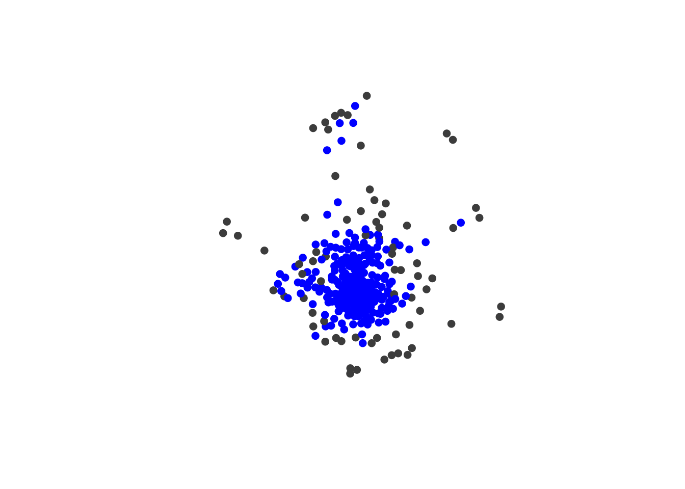

Session Info

sessionInfo()

## R version 4.1.0 (2021-05-18)
## Platform: x86_64-apple-darwin17.0 (64-bit)
## Running under: macOS Big Sur 10.16
## 
## Matrix products: default
## BLAS:   /Library/Frameworks/R.framework/Versions/4.1/Resources/lib/libRblas.dylib
## LAPACK: /Library/Frameworks/R.framework/Versions/4.1/Resources/lib/libRlapack.dylib
## 
## locale:
## [1] en_US.UTF-8/en_US.UTF-8/en_US.UTF-8/C/en_US.UTF-8/en_US.UTF-8
## 
## attached base packages:
## [1] stats     graphics  grDevices utils     datasets  methods   base     
## 
## other attached packages:
## [1] igraph_1.2.6   magrittr_2.0.1 CoDiNA_1.1.2   wTO_1.6.3     
## 
## loaded via a namespace (and not attached):
##  [1] Rcpp_1.0.6        knitr_1.33        som_0.3-5.1       R6_2.5.0         
##  [5] rlang_0.4.11      highr_0.9         stringr_1.4.0     plyr_1.8.6       
##  [9] visNetwork_2.0.9  tools_4.1.0       parallel_4.1.0    data.table_1.14.0
## [13] xfun_0.23         jquerylib_0.1.4   htmltools_0.5.1.1 yaml_2.2.1       
## [17] digest_0.6.27     bookdown_0.22     reshape2_1.4.4    htmlwidgets_1.5.3
## [21] sass_0.4.0        evaluate_0.14     rmarkdown_2.8.5   blogdown_1.3     
## [25] stringi_1.6.2     compiler_4.1.0    bslib_0.2.5.1     jsonlite_1.7.2   
## [29] pkgconfig_2.0.3

References

Morselli Gysi, Deisy, Andre Voigt, Tiago de Miranda Fragoso, Eivind Almaas, and Katja Nowick. 2017. wTO: Computing Weighted Topological Overlaps (wTO) & Consensus wTO Network. https://CRAN.R-project.org/package=wTO.

Gysi, D. M., Fragoso, T.M, Zebardast, F., Beroli, W., Busskamp, V., Almaas, E., Nowick, K. (2018). Whole transcriptomic network analysis using Co-expression Differential Network Analysis (CoDiNA). Plos One, https://doi.org/10.1371/journal.pone.0240523

Sun, Lixin, Ai-Min Hui, Qin Su, Alexander Vortmeyer, Yuri Kotliarov, Sandra Pastorino, Antonino Passaniti, et al. 2006. “Neuronal and Glioma-Derived Stem Cell Factor Induces Angiogenesis Within the Brain.” Cancer Cell 9 (4). Elsevier: 287–300.