wTO
Computing Weighted Topological Overlaps (wTO) & Consensus wTO Network
By Deisy Morselli Gysi in r packages co-expression networks
November 17, 2018
wTO: Computing Weighted Topological Overlaps (wTO) & Consensus wTO Network
Computes the Weighted Topological Overlap with positive and negative signs (wTO) networks (Nowick et al. (2009) doi:10.1073/pnas.0911376106) given a data frame containing the mRNA count/ expression/ abundance per sample, and a vector containing the interested nodes of interaction (a subset of the elements of the full data frame).
It also computes the cut-off threshold or p-value based on the individuals bootstrap or the values reshuffle per individual (Gysi et al. 2017 https://doi.org/10.1186/s12859-018-2351-7). It also allows the construction of a consensus network, based on multiple wTO networks. The package includes a visualization tool for the networks.
You can download the package from CRAN using:
install.packages('wTO')
Input data
The wTO package, can be used on any kind of count data, but we highly
recommend to use normalized and quality controlled data according to the
data type such as RMA, MD5 for microarray, RPKM, TPM or PKM for RNA-seq,
sample normalized data for metagenomics.
As an example, the package contains three data sets, two from microarray
chips (Microarray_Expression1 and Microarray_Expression2), and one
from abundance in metagenomics (metagenomics_abundance).
wTO
The wTO method is a method for building networks based on pairwise correlations normalized and corrected by all shared correlations. For this reason, the user can choose a set of factors of interest, called here Overlaps, those are the nodes that will be corrected and normalized by all other factors in the dataset. Those factors can be Transcription Factor, long non coding RNAs, a set of species of interest etc.
Genomic data
The wTO package contains 2 data sets that were obtained using
expression arrays (Microarray_Expression1 and
Microarray_Expression2), they were previously normalized and the
quality control was done. We will use it to build the wTO network using
the different methods implemented in the package.
First we are going to inspect those data sets.
require(wTO)## Loading required package: wTOrequire(magrittr)## Loading required package: magrittrdata("ExampleGRF")
data("Microarray_Expression1")
data("Microarray_Expression2")
dim(Microarray_Expression1)## [1] 268 18dim(Microarray_Expression2)## [1] 268 18Microarray_Expression1[1:5,1:5]## ID1 ID2 ID3 ID4 ID5
## FAM122B 5.325653 5.039814 5.099828 5.053185 5.213816
## DEFB108B 2.038747 1.965599 1.925807 1.977435 2.079381
## CCSER2 4.973347 4.865783 4.818910 5.024392 4.697314
## GPD2 5.453287 5.595471 5.223886 5.130226 5.370672
## HECW1 4.350837 4.279759 4.218375 4.472152 4.408025head(ExampleGRF)## x
## 1 ACAD8
## 2 ANAPC2
## 3 ANKRD22
## 4 ANKRD2
## 5 ARHGAP35
## 6 ASH1LPlease, note that the individuals are in the columns and the gene expressions are in the rows. Moreover, the row.names() are the names
of the genes. The list of genes that will be used for measuring the
interactions are in ExampleGRF. There should always be more than 2 of
them contained in the expression set. If there are no common nodes to be
measured, the method will return an error.
sum(ExampleGRF$x %in% row.names(Microarray_Expression1))## [1] 168Running the wTO
We can run the wTO package with 3 modes. The first one is running the
wTO without resampling. For that we can use the wTO() . The second
one, wTO.Complete(), gives you the whole diagnosis plot,
hard-threshold on the ωi, j, the
ωi, j, |ωi, j| values and p-values.
The last mode, wTO.fast(), just returns the ωi, j
values and p-value.
Using the wTO() function:
To use the wTO() function, the first step is to compute the
correlation among the nodes of interest using CorrelationOverlap() and
then use it as input for the wTO(). In the first function the user is
allowed to choose the method for correlation between Pearson (‘p’) or
Spearman (‘s’). The second function allows the choice between absolute
values (‘abs’) or signed values (‘sign’). Please, keep in mind that the
result of the wTO() function is a matrix, and it can be easily
converted to an edge list using the function wTO.in.line().
wTO_p_abs = CorrelationOverlap(Data = Microarray_Expression1,
                               Overlap = ExampleGRF$x,
                               method = 'p') %>%
  wTO(., sign = 'abs')
wTO_p_abs[1:5,1:5]
## ZNF333 ZNF28 ANKRD22 ZFR TRIM33
## ZNF333 0.352 0.237 0.269 0.242 0.241
## ZNF28 0.237 0.287 0.209 0.206 0.239
## ANKRD22 0.269 0.209 0.299 0.199 0.252
## ZFR 0.242 0.206 0.199 0.328 0.258
## TRIM33 0.241 0.239 0.252 0.258 0.361wTO_p_abs %<>%
wTO.in.line()
head(wTO_p_abs)## Node.1 Node.2 wTO
## 1: ZNF333 ZNF28 0.237
## 2: ZNF333 ANKRD22 0.269
## 3: ZNF28 ANKRD22 0.209
## 4: ZNF333 ZFR 0.242
## 5: ZNF28 ZFR 0.206
## 6: ANKRD22 ZFR 0.199wTO_s_abs = CorrelationOverlap(Data = Microarray_Expression1,
Overlap = ExampleGRF$x,
method = 's') %>%
wTO(., sign = 'abs') %>%
wTO.in.line()
head(wTO_s_abs)## Node.1 Node.2 wTO
## 1: ZNF333 ZNF28 0.236
## 2: ZNF333 ANKRD22 0.258
## 3: ZNF28 ANKRD22 0.215
## 4: ZNF333 ZFR 0.264
## 5: ZNF28 ZFR 0.187
## 6: ANKRD22 ZFR 0.193wTO_p_sign = CorrelationOverlap(Data = Microarray_Expression1,
Overlap = ExampleGRF$x,
method = 'p') %>%
wTO(., sign = 'sign') %>%
wTO.in.line()
head(wTO_p_sign)## Node.1 Node.2 wTO
## 1: ZNF333 ZNF28 -0.099
## 2: ZNF333 ANKRD22 -0.185
## 3: ZNF28 ANKRD22 0.076
## 4: ZNF333 ZFR -0.117
## 5: ZNF28 ZFR -0.077
## 6: ANKRD22 ZFR -0.036wTO_s_sign = CorrelationOverlap(Data = Microarray_Expression1,
Overlap = ExampleGRF$x,
method = 's') %>%
wTO(., sign = 'sign') %>%
wTO.in.line()
head(wTO_s_sign)## Node.1 Node.2 wTO
## 1: ZNF333 ZNF28 -0.064
## 2: ZNF333 ANKRD22 -0.143
## 3: ZNF28 ANKRD22 0.029
## 4: ZNF333 ZFR -0.164
## 5: ZNF28 ZFR -0.011
## 6: ANKRD22 ZFR 0.024Using the wTO.Complete() function:
The usage of the function wTO.Complete() is straight-forward. No
plug-in-functions() are necessary. The arguments parsed to the
wTO.Complete() functions are the number k of threads that should be
used for computing the ωi,j, the amount of
replications, n, the expression matrix, Data, the Overlapping
nodes, the correlation method (Pearson or Spearman) for the
method_resampling that should be Bootstrap, BlockBootstrap or
Reshuffle, the p-value correction method, pvalmethod (any from the
p.adjust.methods), if the correlation should be saved, the δ is the
expected difference, expected.diff, between the resampled values and
the ωi, j and also if the diagnosis plot should be
plotted.
wTO_s_sign_complete = wTO.Complete(k = 5,
                                   n = 250,
                                   Data = Microarray_Expression1,
                                   Overlap = ExampleGRF$x,
                                   method = 'p',
                                   method_resampling = 'Bootstrap',
                                   pvalmethod = 'BH',
                                   savecor = TRUE,
                                   expected.diff = 0.2,
                                   plot = TRUE)
## There are 168 overlapping nodes, 268 total nodes and 18 individuals.## This function might take a long time to run. Don't turn off the computer.## Simulations are done.## Computing p-values## Computing cutoffs## Done!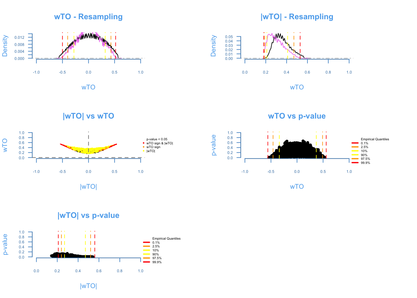
The diagnosis plot shows the quality of the resampling (first two plots). The closer the purple line to the black line, the better. The ωi,j vs |ωi,j| shows the amount of ωi, j being affected by cancellations on the heuristics of the method, the more similar to a smile plot, the better. The last two plots show the relashionship between p-values and the ωi,j. It is expected that higher ω’s presents lower p-values.
The resulting object from the wTO.Complete() function is a list
containing:
* wTO an edge list of informations such as the signed and
unsigned ωi,j values its raw and adjusted p-values.
* Correlation values, also as an edge list
* Quantiles, the quantiles from the empirical distribution and the calculated ω’s from the
original data, for both signed and unsigned networks.
wTO_s_sign_complete## $wTO
## Node.1 Node.2 wTO_sign wTO_abs pval_sig pval_abs Padj_sig Padj_abs
## 1: ZNF333 ZNF28 -0.099 0.237 0.152 0.012 0.3472353 0.02018417
## 2: ZNF333 ANKRD22 -0.185 0.269 0.184 0.004 0.3472353 0.01092311
## 3: ZNF333 ZFR -0.117 0.242 0.116 0.016 0.3472353 0.02361368
## 4: ZNF333 TRIM33 0.007 0.241 0.136 0.008 0.3472353 0.01629268
## 5: ZNF333 RIMS3 -0.325 0.409 0.140 0.000 0.3472353 0.00000000
## ---
## 14024: ANAPC2 SBNO2 -0.147 0.298 0.160 0.000 0.3472353 0.00000000
## 14025: ANAPC2 ZNF528 -0.142 0.222 0.164 0.004 0.3472353 0.01092311
## 14026: TIGD7 SBNO2 -0.297 0.354 0.104 0.000 0.3472353 0.00000000
## 14027: TIGD7 ZNF528 -0.099 0.219 0.152 0.020 0.3472353 0.02684014
## 14028: SBNO2 ZNF528 0.141 0.311 0.272 0.008 0.3554039 0.01629268
##
## $Correlation
## Node.1 Node.2 Cor
## 1: FAM122B DEFB108B 0.366857931
## 2: FAM122B CCSER2 0.278870911
## 3: DEFB108B CCSER2 -0.252482453
## 4: FAM122B GPD2 -0.005649124
## 5: DEFB108B GPD2 -0.107064848
## ---
## 35774: TRIM23 ZNF528 0.054249174
## 35775: ZNF559 ZNF528 -0.218309729
## 35776: ANAPC2 ZNF528 -0.013821370
## 35777: TIGD7 ZNF528 0.011807143
## 35778: SBNO2 ZNF528 0.092317502
##
## $Quantiles
## 0.1% 2.5% 10% 90% 97.5% 99.9%
## Empirical.Quantile -0.56 -0.46 -0.34 0.37 0.49 0.56
## Quantile -0.50 -0.40 -0.28 0.32 0.43 0.52
## Empirical.Quantile.abs 0.21 0.24 0.27 0.47 0.52 0.56
## Quantile.abs 0.18 0.19 0.21 0.41 0.47 0.53
##
## attr(,"class")
## [1] "wTO" "list"Using the wTO.fast() function:
The wTO.fast() function is a simplified verion of the wTO.Complete()
function, that doesn’t return diagnosis, correlation, nor the quantiles,
but allows the user to choose the method for correlation, the sign of
the ω to be calculated and the resampling method should be one of the
two Bootrastap or BlockBootstrap. The p-values are the raw
p-values and if the user desires to calculate its correction it can be
easily done as shown above.
fast_example = wTO.fast(Data = Microarray_Expression1,
                        Overlap = ExampleGRF$x,
                        method = 's',
                        sign = 'sign',
                        delta = 0.2,
                        n = 250,
                        method_resampling = 'Bootstrap')
## There are 168 overlapping nodes, 268 total nodes and 18 individuals.## This function might take a long time to run. Don't turn off the computer.## 1 2 3 4 5 6 7 8 9 10 11 12 13 14 15 16 17 18 19 20 21 22 23 24 25 26 27 28 29 30 31 32 33 34 35 36 37 38 39 40 41 42 43 44 45 46 47 48 49 50 51 52 53 54 55 56 57 58 59 60 61 62 63 64 65 66 67 68 69 70 71 72 73 74 75 76 77 78 79 80 81 82 83 84 85 86 87 88 89 90 91 92 93 94 95 96 97 98 99 100 101 102 103 104 105 106 107 108 109 110 111 112 113 114 115 116 117 118 119 120 121 122 123 124 125 126 127 128 129 130 131 132 133 134 135 136 137 138 139 140 141 142 143 144 145 146 147 148 149 150 151 152 153 154 155 156 157 158 159 160 161 162 163 164 165 166 167 168 169 170 171 172 173 174 175 176 177 178 179 180 181 182 183 184 185 186 187 188 189 190 191 192 193 194 195 196 197 198 199 200 201 202 203 204 205 206 207 208 209 210 211 212 213 214 215 216 217 218 219 220 221 222 223 224 225 226 227 228 229 230 231 232 233 234 235 236 237 238 239 240 241 242 243 244 245 246 247 248 249 250 Done!head(fast_example)## Node.1 Node.2 wTO pval pval.adj
## 1: ZNF333 ZNF28 -0.064 0.272 0.4363894
## 2: ZNF333 ANKRD22 -0.143 0.308 0.4363894
## 3: ZNF28 ANKRD22 0.029 0.224 0.4363894
## 4: ZNF333 ZFR -0.164 0.200 0.4363894
## 5: ZNF28 ZFR -0.011 0.336 0.4363894
## 6: ANKRD22 ZFR 0.024 0.284 0.4363894fast_example$adj.pval = p.adjust(fast_example$pval)Metagenomic data
Along with the expression data, the wTO package also includes a
metagenomics dataset that is the abundance of some OTU’s in bacterias
collected since 1997. More about this data can be found at
\[<https://www.ebi.ac.uk/metagenomics/projects/ERP013549>\].
The OTU (Operational Taxonomic Units) contains the taxonomy of the particular OTU and from Week1 to Week98, the abundance of that particular OTU in that week.
data("metagenomics_abundance")
metagenomics_abundance[2:10, 1:10]
## OTU
## 2 Root;k__Archaea;p__Euryarchaeota;c__Thermoplasmata;o__E2;f__MarinegroupII;g__;s__
## 3 Root;k__Bacteria;p__Actinobacteria;c__Acidimicrobiia;o__Acidimicrobiales;f__OCS155;g__;s__
## 4 Root;k__Bacteria;p__Actinobacteria;c__Actinobacteria;o__Actinomycetales;f__Microbacteriaceae;g__;s__
## 5 Root;k__Bacteria;p__Bacteroidetes;c__Cytophagia;o__Cytophagales;f__Flammeovirgaceae;g__;s__
## 6 Root;k__Bacteria;p__Bacteroidetes;c__Cytophagia;o__Cytophagales;f__Flammeovirgaceae;g__JTB248;s__
## 7 Root;k__Bacteria;p__Bacteroidetes;c__Flavobacteriia;o__Flavobacteriales;f__;g__;s__
## 8 Root;k__Bacteria;p__Bacteroidetes;c__Flavobacteriia;o__Flavobacteriales;f__Cryomorphaceae;g__;s__
## 9 Root;k__Bacteria;p__Bacteroidetes;c__Flavobacteriia;o__Flavobacteriales;f__Cryomorphaceae;g__Fluviicola;s__
## 10 Root;k__Bacteria;p__Bacteroidetes;c__Flavobacteriia;o__Flavobacteriales;f__Flavobacteriaceae;g__;s__
## Week1 Week2 Week3 Week4 Week5 Week6 Week7 Week8 Week9
## 2 1 6 0 0 0 1 0 1 0
## 3 0 0 0 0 0 0 0 5 0
## 4 0 0 0 0 0 0 0 0 0
## 5 0 1 0 0 0 0 0 0 0
## 6 0 0 0 0 0 0 0 0 0
## 7 0 1 0 0 0 0 0 1 0
## 8 0 0 0 0 0 0 0 1 0
## 9 0 0 0 0 0 0 0 1 0
## 10 0 1 0 0 0 0 0 7 0Before we are able to define the network, we have first to understand
the patterns of autocorrelation of each species, and then define the
lag, that will be used for the BlockBootstrap resampling in the
wTO.Complete() or fast.wTO() functions. To define the lag, we use
autocorrelation function acf().
row.names(metagenomics_abundance) = metagenomics_abundance$OTU
metagenomics_abundance = metagenomics_abundance[,-1]
par(mfrow = c(3,3))
for ( i in 1:nrow(metagenomics_abundance)){
  acf(t(metagenomics_abundance[i,]))
}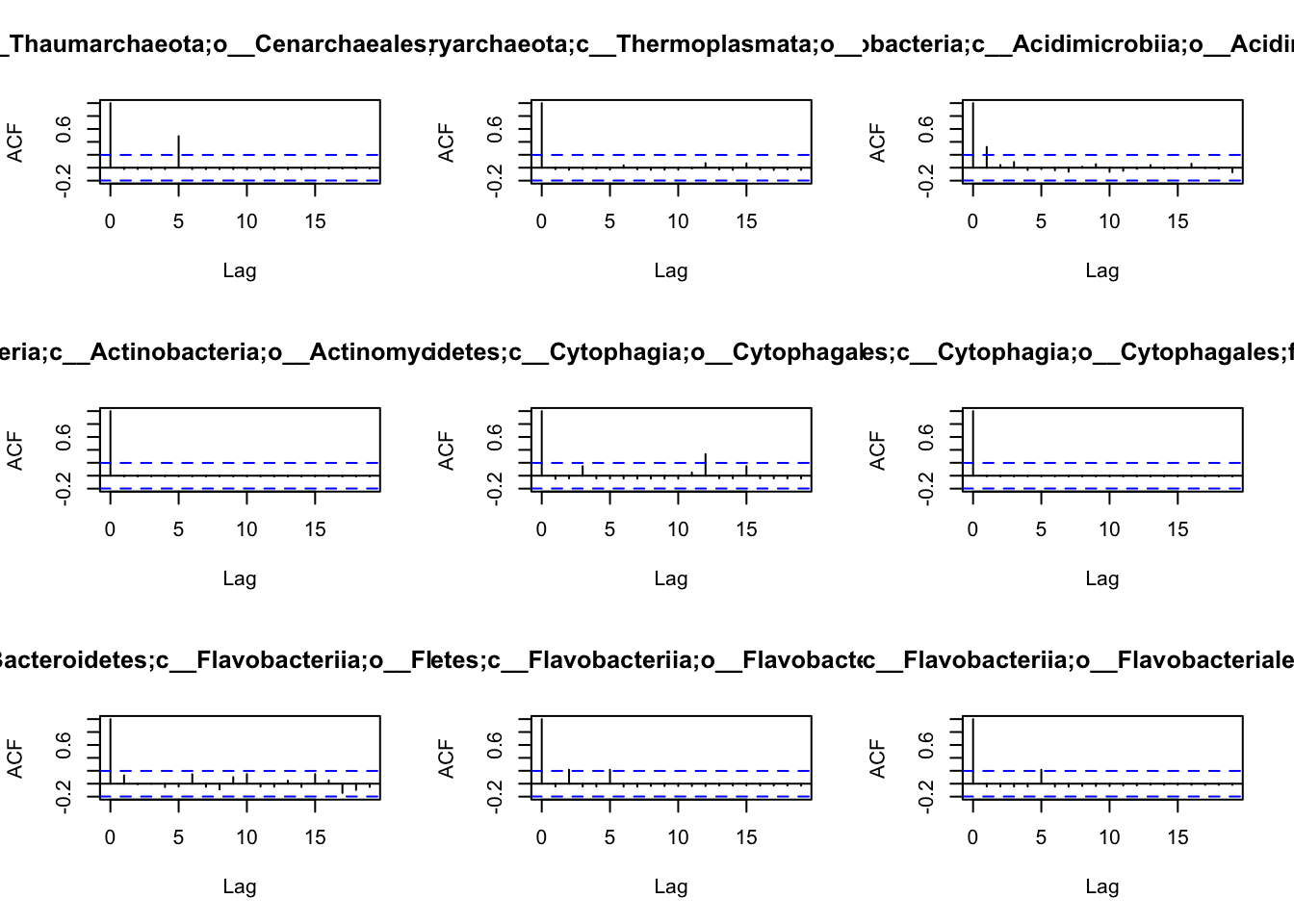
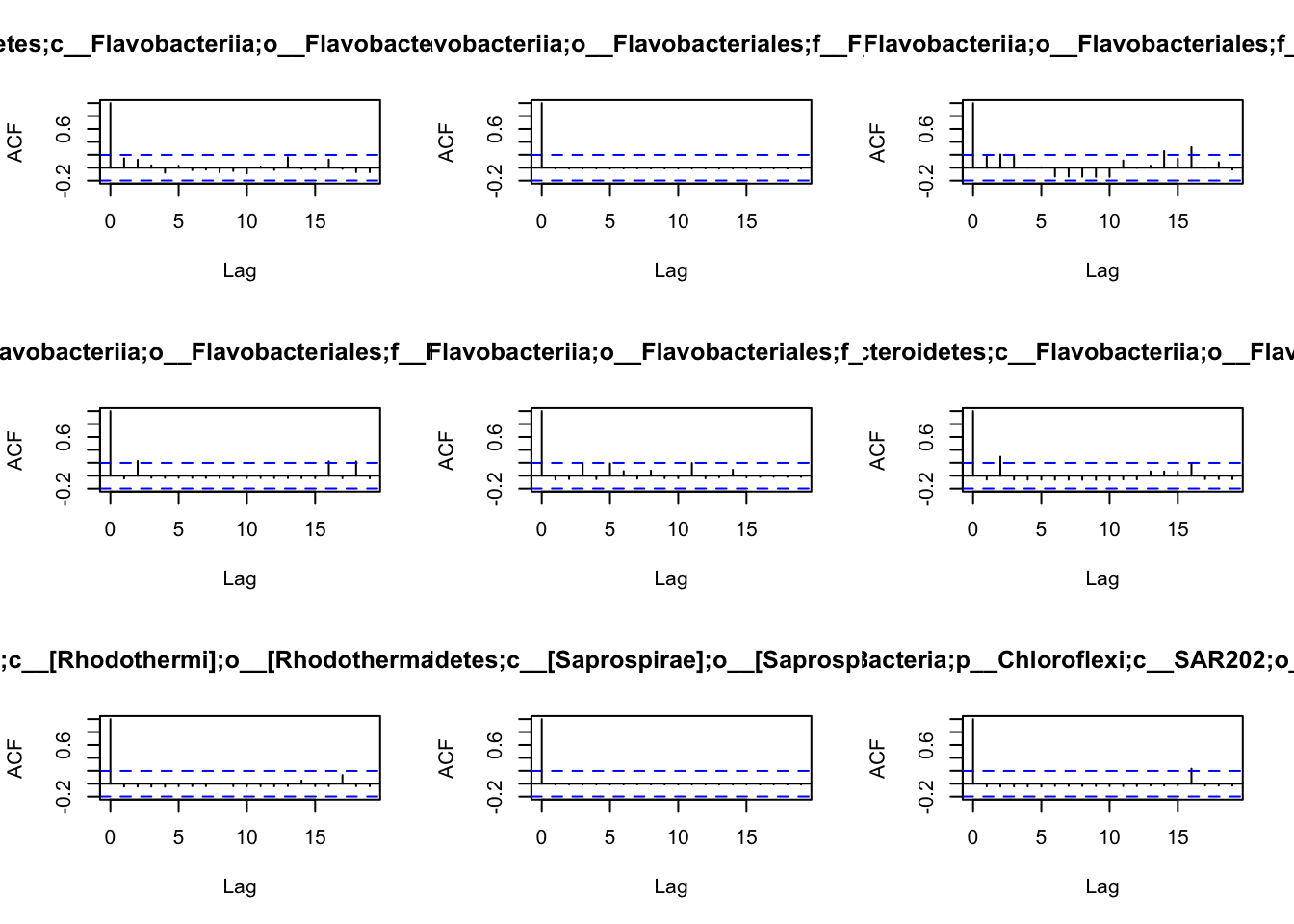
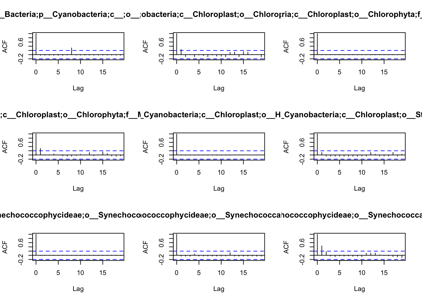
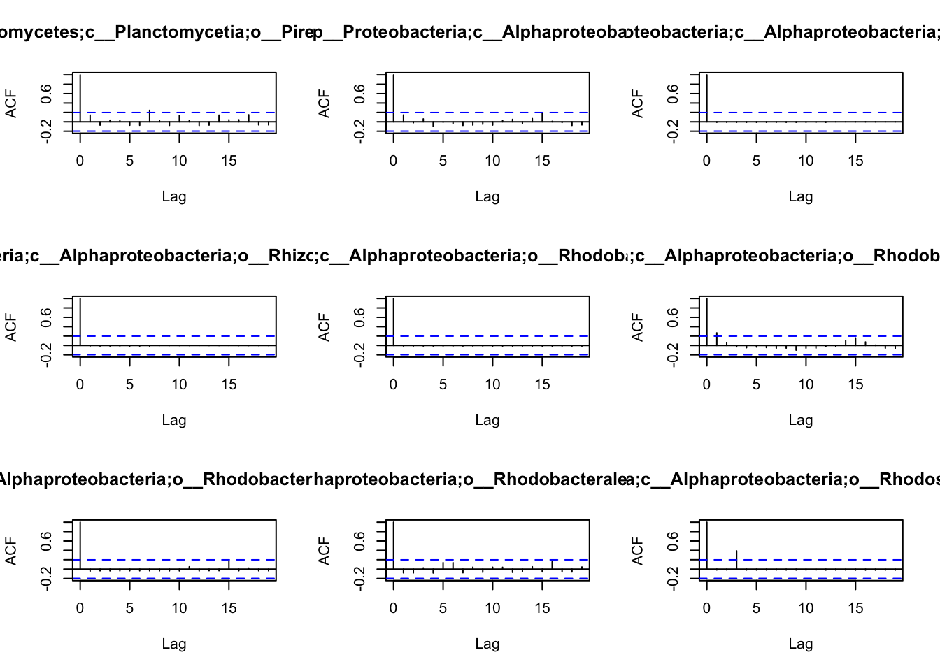
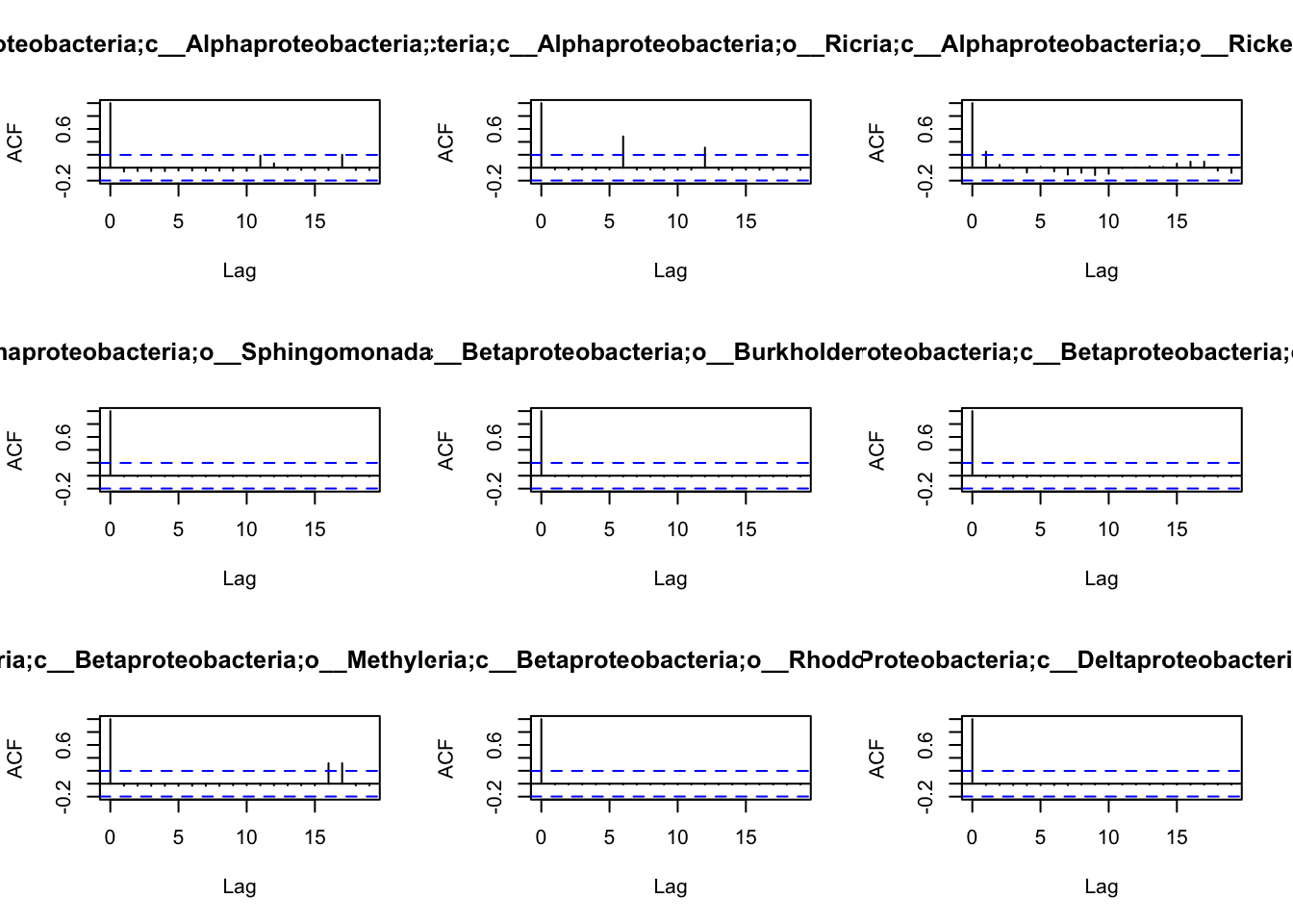
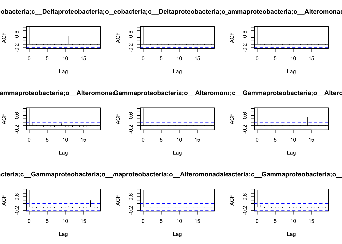
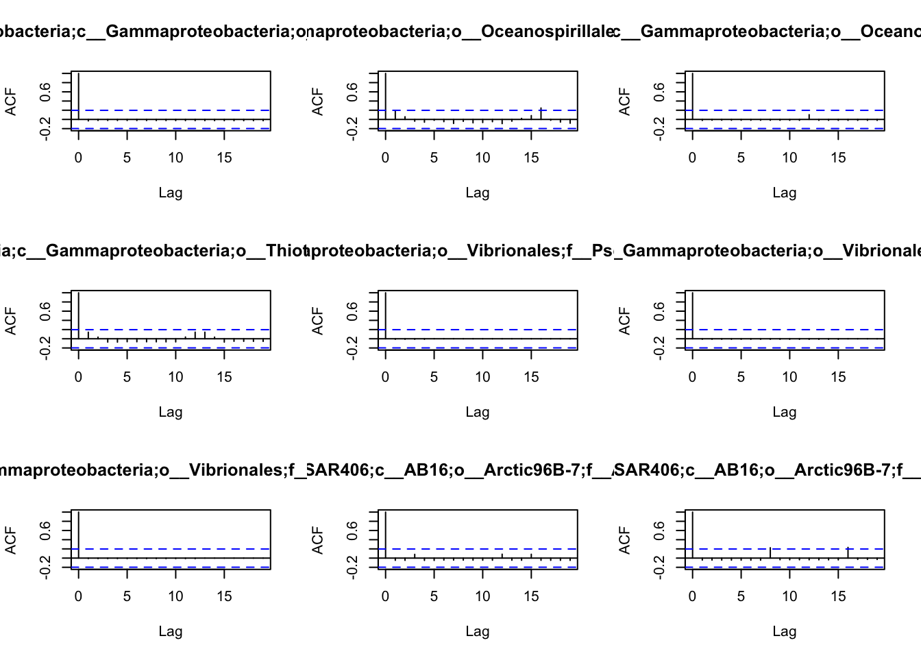
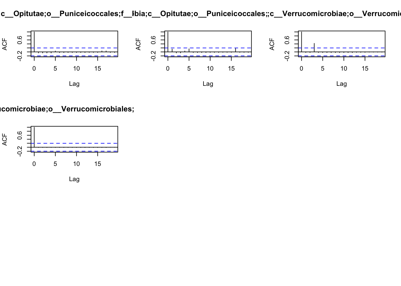
Because most of them have only a high autocorrelation with itself or maximum 2 weeks, we will use a lag of 2 for the blocks used in the bootstrap.
The functions wTO.fast() and wTO.Complete() are able to accomodate
the lag parameter, therefore, they will be used here.
Meta_fast = wTO.fast(Data = metagenomics_abundance,
                     Overlap = row.names(metagenomics_abundance),
                     method = 'p',
                     sign = 'sign',
                     n = 250,
                     method_resampling = 'BlockBootstrap',
                     lag = 2)
## There are 67 overlapping nodes, 67 total nodes and 98 individuals.## This function might take a long time to run. Don't turn off the computer.## 1 2 3 4 5 6 7 8 9 10 11 12 13 14 15 16 17 18 19 20 21 22 23 24 25 26 27 28 29 30 31 32 33 34 35 36 37 38 39 40 41 42 43 44 45 46 47 48 49 50 51 52 53 54 55 56 57 58 59 60 61 62 63 64 65 66 67 68 69 70 71 72 73 74 75 76 77 78 79 80 81 82 83 84 85 86 87 88 89 90 91 92 93 94 95 96 97 98 99 100 101 102 103 104 105 106 107 108 109 110 111 112 113 114 115 116 117 118 119 120 121 122 123 124 125 126 127 128 129 130 131 132 133 134 135 136 137 138 139 140 141 142 143 144 145 146 147 148 149 150 151 152 153 154 155 156 157 158 159 160 161 162 163 164 165 166 167 168 169 170 171 172 173 174 175 176 177 178 179 180 181 182 183 184 185 186 187 188 189 190 191 192 193 194 195 196 197 198 199 200 201 202 203 204 205 206 207 208 209 210 211 212 213 214 215 216 217 218 219 220 221 222 223 224 225 226 227 228 229 230 231 232 233 234 235 236 237 238 239 240 241 242 243 244 245 246 247 248 249 250 Done!Meta_Complete = wTO.Complete(k = 1,
n = 250,
Data = metagenomics_abundance,
Overlap = row.names(metagenomics_abundance),
method = 's' ,
method_resampling = 'BlockBootstrap',
lag = 2 )## There are 67 overlapping nodes, 67 total nodes and 98 individuals.
## This function might take a long time to run. Don't turn off the computer.
## Simulations are done.
## Computing p-values
## Computing cutoffs
## Done!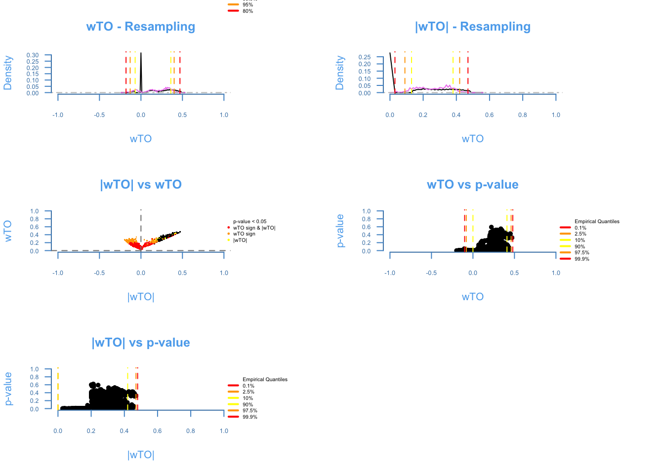
Consensus Network
From the expression data-sets, we are able to draw a Consensus Network.
For that, the function wTO.Consensus() can be used. This function
works in a special way, that the user should pass a list of data.frames
containing the Nodes names and the wTO and p-values. We show an example
above.
Let’s calculate the networks the same way we did in the Section Genomic data.
wTO_Data1 = wTO.fast(Data = Microarray_Expression1,
                     Overlap = ExampleGRF$x,
                     method = 'p',
                     n = 250)
## There are 168 overlapping nodes, 268 total nodes and 18 individuals.## This function might take a long time to run. Don't turn off the computer.## 1 2 3 4 5 6 7 8 9 10 11 12 13 14 15 16 17 18 19 20 21 22 23 24 25 26 27 28 29 30 31 32 33 34 35 36 37 38 39 40 41 42 43 44 45 46 47 48 49 50 51 52 53 54 55 56 57 58 59 60 61 62 63 64 65 66 67 68 69 70 71 72 73 74 75 76 77 78 79 80 81 82 83 84 85 86 87 88 89 90 91 92 93 94 95 96 97 98 99 100 101 102 103 104 105 106 107 108 109 110 111 112 113 114 115 116 117 118 119 120 121 122 123 124 125 126 127 128 129 130 131 132 133 134 135 136 137 138 139 140 141 142 143 144 145 146 147 148 149 150 151 152 153 154 155 156 157 158 159 160 161 162 163 164 165 166 167 168 169 170 171 172 173 174 175 176 177 178 179 180 181 182 183 184 185 186 187 188 189 190 191 192 193 194 195 196 197 198 199 200 201 202 203 204 205 206 207 208 209 210 211 212 213 214 215 216 217 218 219 220 221 222 223 224 225 226 227 228 229 230 231 232 233 234 235 236 237 238 239 240 241 242 243 244 245 246 247 248 249 250 Done!wTO_Data2 = wTO.fast(Data = Microarray_Expression2,
Overlap = ExampleGRF$x,
method = 'p',
n = 250)## There are 168 overlapping nodes, 268 total nodes and 18 individuals.
## This function might take a long time to run. Don't turn off the computer.
## 1 2 3 4 5 6 7 8 9 10 11 12 13 14 15 16 17 18 19 20 21 22 23 24 25 26 27 28 29 30 31 32 33 34 35 36 37 38 39 40 41 42 43 44 45 46 47 48 49 50 51 52 53 54 55 56 57 58 59 60 61 62 63 64 65 66 67 68 69 70 71 72 73 74 75 76 77 78 79 80 81 82 83 84 85 86 87 88 89 90 91 92 93 94 95 96 97 98 99 100 101 102 103 104 105 106 107 108 109 110 111 112 113 114 115 116 117 118 119 120 121 122 123 124 125 126 127 128 129 130 131 132 133 134 135 136 137 138 139 140 141 142 143 144 145 146 147 148 149 150 151 152 153 154 155 156 157 158 159 160 161 162 163 164 165 166 167 168 169 170 171 172 173 174 175 176 177 178 179 180 181 182 183 184 185 186 187 188 189 190 191 192 193 194 195 196 197 198 199 200 201 202 203 204 205 206 207 208 209 210 211 212 213 214 215 216 217 218 219 220 221 222 223 224 225 226 227 228 229 230 231 232 233 234 235 236 237 238 239 240 241 242 243 244 245 246 247 248 249 250 Done!Now, let’s combine both networks in one Consensus Network.
CN_expression = wTO.Consensus(data = list (wTO_Data1 = data.frame
                                           (Node.1 = wTO_Data1$Node.1,
                                             Node.2 = wTO_Data1$Node.2,
                                             wTO = wTO_Data1$wTO,
                                             pval = wTO_Data1$pval)
                                           , wTO_Data2C = data.frame
                                           (Node.1 = wTO_Data2$Node.1,
                                             Node.2 = wTO_Data2$Node.2,
                                             wTO = wTO_Data2$wTO,
                                             pval = wTO_Data2$pval)))
## Joining by: Node.1, Node.2
## Joining by: Node.1, Node.2## Joining by: ID## Total common nodes: 168Or using the wTO.Complete():
wTO_Data1C = wTO.Complete(Data = Microarray_Expression1,
                          Overlap = ExampleGRF$x,
                          method = 'p',
                          n = 250,
                          k = 5)
## There are 168 overlapping nodes, 268 total nodes and 18 individuals.## This function might take a long time to run. Don't turn off the computer.## Simulations are done.## Computing p-values## Computing cutoffs## Done!wTO_Data2C = wTO.Complete(Data = Microarray_Expression2,
Overlap = ExampleGRF$x,
method = 'p',
n = 250,
k = 5)## There are 168 overlapping nodes, 268 total nodes and 18 individuals.## This function might take a long time to run. Don't turn off the computer.## Simulations are done.## Computing p-values## Computing cutoffs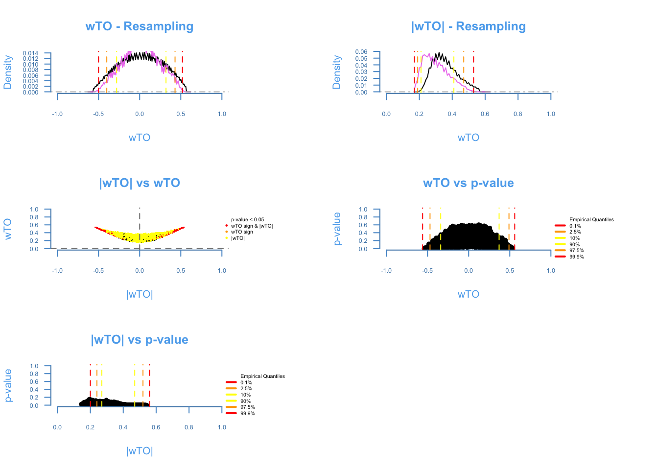
## Done!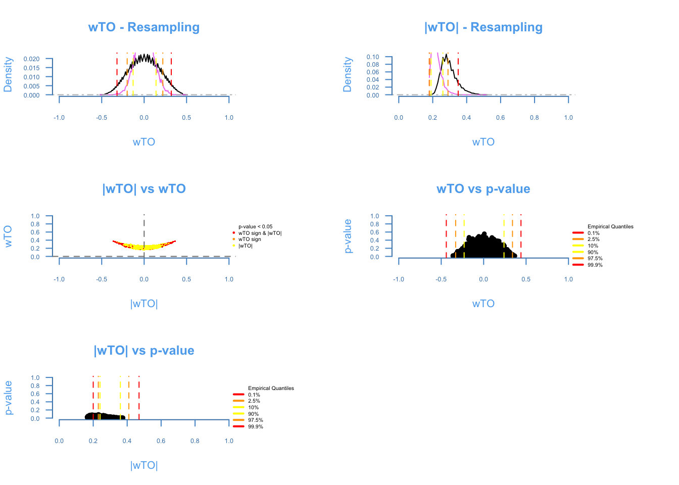
Now, let’s combine both networks in one Consensus Network.
CN_expression = wTO.Consensus(data = list (wTO_Data1C = data.frame
                                           (Node.1 = wTO_Data1C$wTO$Node.1,
                                             Node.2 = wTO_Data1C$wTO$Node.2,
                                             wTO = wTO_Data1C$wTO$wTO_sign,
                                             pval = wTO_Data1C$wTO$pval_sig), wTO_Data2C = data.frame
                                           (Node.1 = wTO_Data2C$wTO$Node.1,
                                             Node.2 = wTO_Data2C$wTO$Node.2,
                                             wTO = wTO_Data2C$wTO$wTO_sign,
                                             pval = wTO_Data2C$wTO$pval_sig)))
## Joining by: Node.1, Node.2
## Joining by: Node.1, Node.2## Joining by: ID## Total common nodes: 168head(CN_expression)## Node.1 Node.2 CN pval.fisher
## 1 ZNF333 ZNF28 -0.1191288 0.08584314
## 2 ZNF333 ANKRD22 -0.1400000 0.11936952
## 3 ZNF333 ZFR -0.1091659 0.09698604
## 4 ZNF333 TRIM33 -0.0240000 0.06464921
## 5 ZNF333 RIMS3 -0.2798101 0.09711171
## 6 ZNF333 ZNF595 0.1542850 0.12426164Visualization
The wTO package also includes an interactive visualization tool that
can be used to inspect the results of the wTO netwoks or Consensus
Network.
The arguments given to this function are the Nodes names, its wTO and
p-values. Optionals are the cutoffs that can be applied to the p-value
or to the wTO value. We highly reccomend using both by subseting the
data previous to the visualization. The layout of the network can be
also chosen from a variety that are implemented in igraph package, for
the the Make_Cluster argument many clustering algorithms that are
implemented in igraph can be used. The final graph can be exported as an
html or as png.
Visualization = NetVis(Node.1 = CN_expression$Node.1,
                       Node.2 = CN_expression$Node.2,
                       wTO = CN_expression$CN,
                       pval = CN_expression$pval.fisher,
                       cutoff = list(kind = 'pval', value = 0.001),
                       MakeGroups = 'louvain',
                       layout = 'layout_components')
## Joining by: idCN_expression_filtered = subset(CN_expression,
abs(CN_expression$CN)> 0.4 &
CN_expression$pval.fisher < 0.0001)
dim(CN_expression_filtered)## [1] 50 4Visualization2 = NetVis(
Node.1 = CN_expression_filtered$Node.1,
Node.2 = CN_expression_filtered$Node.2,
wTO = CN_expression_filtered$CN,
pval = CN_expression_filtered$pval.fisher,
cutoff = list(kind = 'pval', value = 0.001),
MakeGroups = 'louvain',
layout = 'layout_components', path = 'Vis.html')## Joining by: id## Vis.htmlSession Info
sessionInfo()## R version 4.1.0 (2021-05-18)
## Platform: x86_64-apple-darwin17.0 (64-bit)
## Running under: macOS Big Sur 10.16
##
## Matrix products: default
## BLAS: /Library/Frameworks/R.framework/Versions/4.1/Resources/lib/libRblas.dylib
## LAPACK: /Library/Frameworks/R.framework/Versions/4.1/Resources/lib/libRlapack.dylib
##
## locale:
## [1] en_US.UTF-8/en_US.UTF-8/en_US.UTF-8/C/en_US.UTF-8/en_US.UTF-8
##
## attached base packages:
## [1] stats graphics grDevices utils datasets methods base
##
## other attached packages:
## [1] magrittr_2.0.1 wTO_1.6.3
##
## loaded via a namespace (and not attached):
## [1] igraph_1.2.6 Rcpp_1.0.6 knitr_1.33 som_0.3-5.1
## [5] R6_2.5.0 rlang_0.4.11 highr_0.9 stringr_1.4.0
## [9] plyr_1.8.6 visNetwork_2.0.9 tools_4.1.0 parallel_4.1.0
## [13] data.table_1.14.0 xfun_0.23 jquerylib_0.1.4 htmltools_0.5.1.1
## [17] yaml_2.2.1 digest_0.6.27 bookdown_0.22 reshape2_1.4.4
## [21] htmlwidgets_1.5.3 sass_0.4.0 evaluate_0.14 rmarkdown_2.8.5
## [25] blogdown_1.3 stringi_1.6.2 compiler_4.1.0 bslib_0.2.5.1
## [29] jsonlite_1.7.2 pkgconfig_2.0.3- Posted on:
- November 17, 2018
- Length:
- 18 minute read, 3778 words
- Categories:
- r packages co-expression networks
- See Also: