Network Analysis for Biological Data
A surviving guide
By Deisy Morselli Gysi in r packages co-expression networks network comparisson network medicine
April 10, 2021
miniPEB 2021: Network Analysis
Link to the course: learnNetSci.
Network Science: Overview
Network Science is broadly employed in many fields: from understanding how friends bond in a party to how animals interact; from how superheroes appear in the same comic books to how genes can be related to a specific biological process. Network analysis is especially beneficial for understanding complex systems, in all research fields. Examples of complex biological or medical systems include gene regulatory, ecological, and neuropsychology networks. In this workshop, the focus is given to applications of Network Science to the Medical Sciences.
Here, I will start by introducing the basic network terminologies and then explore how can we define and identify disease modules, identify disease commorbidities, and lastly, we will learn how to repurpuse drugs for diseases with known modules. For each step, I will then present some classical and some new studies.
It is expected some degree of familiarity with R, ggplot2, tidyr, and igraph.
- How people interact in a party?
- How people interact in a Social Media?
- How genes interact?
Why networks are important?
Networks enable us to understand how interactions between entities can affect an outcome.
How gene interactions can be associated with a disease or trait
How genes can be differentially co-expressed in a phenotype
How drugs target different proteins and can affect drug response
Terminology
While the nature of each system, i.e. what its entities are and what kind of interactions they have, is different, there are common notations.
The set of interactions among a set of entities is, in general, called a graph or a network (Newman 2018; Barabási 2016). In graph theory, each entity is called a vertex, while in network notation it is called a node (Barabási 2016). Accordingly, the connections between two entities are called edges or links, respectively (Barabási 2016). In this workshop, I will always use the network notation, unless otherwise specified. The total number of nodes in a network is often denoted as N, and the number of links in a network is denoted as L. While nodes can receive a label, links in general, are not labeled (Barabási 2016) (although, in many cases, weights can also be perceived as a label).
A network can be represented mathematically as an adjacency matrix (usually denoted as A), an edge-list, or visually as a graph.
- Adjacency matrix:
| A | B | C | D | E | F | G | H | I | J | |
|---|---|---|---|---|---|---|---|---|---|---|
| A | 0 | 1 | 1 | 1 | 1 | 0 | 0 | 0 | 1 | 0 |
| B | 1 | 0 | 0 | 1 | 0 | 1 | 1 | 0 | 0 | 0 |
| C | 1 | 0 | 0 | 0 | 0 | 1 | 0 | 1 | 0 | 1 |
| D | 1 | 1 | 0 | 0 | 0 | 0 | 0 | 0 | 0 | 0 |
| E | 1 | 0 | 0 | 0 | 0 | 0 | 0 | 0 | 0 | 0 |
| F | 0 | 1 | 1 | 0 | 0 | 0 | 0 | 0 | 0 | 0 |
| G | 0 | 1 | 0 | 0 | 0 | 0 | 0 | 0 | 0 | 0 |
| H | 0 | 0 | 1 | 0 | 0 | 0 | 0 | 0 | 0 | 0 |
| I | 1 | 0 | 0 | 0 | 0 | 0 | 0 | 0 | 0 | 0 |
| J | 0 | 0 | 1 | 0 | 0 | 0 | 0 | 0 | 0 | 0 |
- Edge list:
| from | to |
|---|---|
| A | D |
| C | H |
| B | F |
| C | J |
| A | I |
| D | B |
| B | A |
| A | E |
| B | G |
| A | C |
| F | C |
A network is a pair G = (N, L) of a set N of nodes connected by a set L of links.
Two nodes are neighbors if they are connected.
The degree (d) of a node is the number of nodes it interacts with.
Nodes with high degree are called hubs.
The strength of a node is the sum of the weights attached to links belonging to a node.
- Networks come in all sorts of flavors. They can have weights and/ or directions on their edges.
Two nodes are connected in a network, if a sequence of adjacent nodes, a path, connects them.
The shortest path length is the number of links along the shortest path connecting two nodes.
The average path length is the average of the shortest paths between all pairs of nodes.
- An induced subgraph is a subgraph that contains a set of “defined” nodes.
Data Commonly Used in Network Medicine
In Network Medicine, we are often interested in understanding how genes associated to a particular disease can influence each other, how two diseases are similar (or different), and how a drug can be used in different set-ups.
For that, it is necessary to use data sets that are able to represent those associations: Protein-Protein Interactions are used as a map of the interactions inside our cells; Gene-Disease-Associations are used for us to identify genes that were previously associated to diseases, often using a GWAS approach.
Protein-Protein Interaction Networks
In PPI networks, the nodes represent proteins, and they are connected by a link if they physically interact with each other (Rual et al. 2005). Typically, these interactions are measured experimentally, for instance, with the Yeast-Two-Hybrid (Y2H) system (Uetz et al. 2000), or by protein complex immunoprecipitation followed by high-throughput Mass Spectrometry (Zhang et al. 2008; Koh et al. 2012), or inferred computationally based on sequence similarity (Fong, Keating, and Singh 2004). PPI can be used to infer gene functions and the association of sub-networks to diseases (Menche et al. 2015). In this type of network, a highly connected protein tends to interact with proteins that are less connected, probably to prevent unwanted cross-talk of functional modules. Most of the methods in network medicine are based on PPI.
Measuring PPIs
Protein-Protein Interactions can be measured mainly using three different techniques:
By the creation of Protein-Protein interaction maps derived from existing scientific literature;
Using computational predictions of PPIs based on available orthogonal information; and
By systematic experimental mapping of proteins identify complex association and/or binary interactions.
Commonly used data sources for PPIs
PPIs can be found from different sources. I list here some well-known databases for that.
- Binary PPIs derived from high-throughput yeast-two hybrid (Y2H) experiments;
- Binary PPIs three-dimensional (3D) protein structures;
- Binary PPIs literature curation;
- PPIs identified by affinity purification followed by mass spectrometry;
- Kinase substrate interactions;
- Signaling interactions;
- Regulatory interactions.
Understanding a PPI
For this workshop, we will be using for this workshop is a combination of a manually curated PPI that combines all previous data sets. The data can be found here. This PPI was previously published in D. M. Gysi et al. (2020).
Before we can start any analysis using this interactome, let us first understand this data.
The PPI contains the EntrezID and the HGNC symbol of each gene, and some might not have a proper map. Therefore, it should be removed from further analysis. Moreover, we might have loops, and those should also be removed.
Let us begin by preparing our environment and calling all libraries we will need at this point.
require(data.table)
require(tidyr)
require(igraph)
require(dplyr)
require(magrittr)
require(ggplot2)
Let’s read in our data.
PPI = fread("./data/PPI_Symbol_Entrez.csv")

head(PPI)
## GeneA_ID GeneB_ID Symbol_A Symbol_B
## 1: 9796 56992 PHYHIP KIF15
## 2: 7918 9240 GPANK1 PNMA1
## 3: 8233 23548 ZRSR2 TTC33
## 4: 4899 11253 NRF1 MAN1B1
## 5: 5297 8601 PI4KA RGS20
## 6: 6564 8933 SLC15A1 RTL8CLet’s transform our edge-list into a network.
How many genes do we have? How many interactions?
## IGRAPH d407e14 UN-- 18507 322289 --
## + attr: name (v/c)
## + edges from d407e14 (vertex names):
##  [1] PHYHIP--TTR      PHYHIP--NFE2     PHYHIP--DYRK1A   PHYHIP--HNRNPA1
##  [5] PHYHIP--COPS6    PHYHIP--SUPT5H   PHYHIP--SMARCC2  PHYHIP--EEF1A1
##  [9] PHYHIP--TRIP6    PHYHIP--NDUFV3   PHYHIP--CA10     PHYHIP--ERG28
## [13] PHYHIP--S100A13  PHYHIP--PPIE     PHYHIP--LIMD1    PHYHIP--ANKRD12
## [17] PHYHIP--ZZEF1    PHYHIP--PRMT5    PHYHIP--KIF15    PHYHIP--MED8
## [21] PHYHIP--PRKD2    PHYHIP--PAQR5    PHYHIP--MAGED4B  PHYHIP--NDRG1
## [25] PHYHIP--PTRH2    PHYHIP--HDAC11   PHYHIP--METTL18  PHYHIP--PNPLA2
## [29] PHYHIP--TMEM255B PHYHIP--WDR89    PHYHIP--FAM131A  GPANK1--TAF1
## + ... omitted several edges
Next, let’s check the degree distribution:
dd = degree(gPPI) %>%
  table() %>%
  as.data.frame()

names(dd) = c('Degree', "Nodes")
dd$Degree %<>% as.character %>% as.numeric()
dd$Nodes  %<>% as.character %>% as.numeric()

ggplot(dd) +
  aes(x = Degree, y = Nodes) +
  geom_point(colour = "#1d3557") +
  scale_x_continuous(trans = "log10") +
  scale_y_continuous(trans = "log10") +
  theme_minimal()
## Warning: Transformation introduced infinite values in continuous x-axis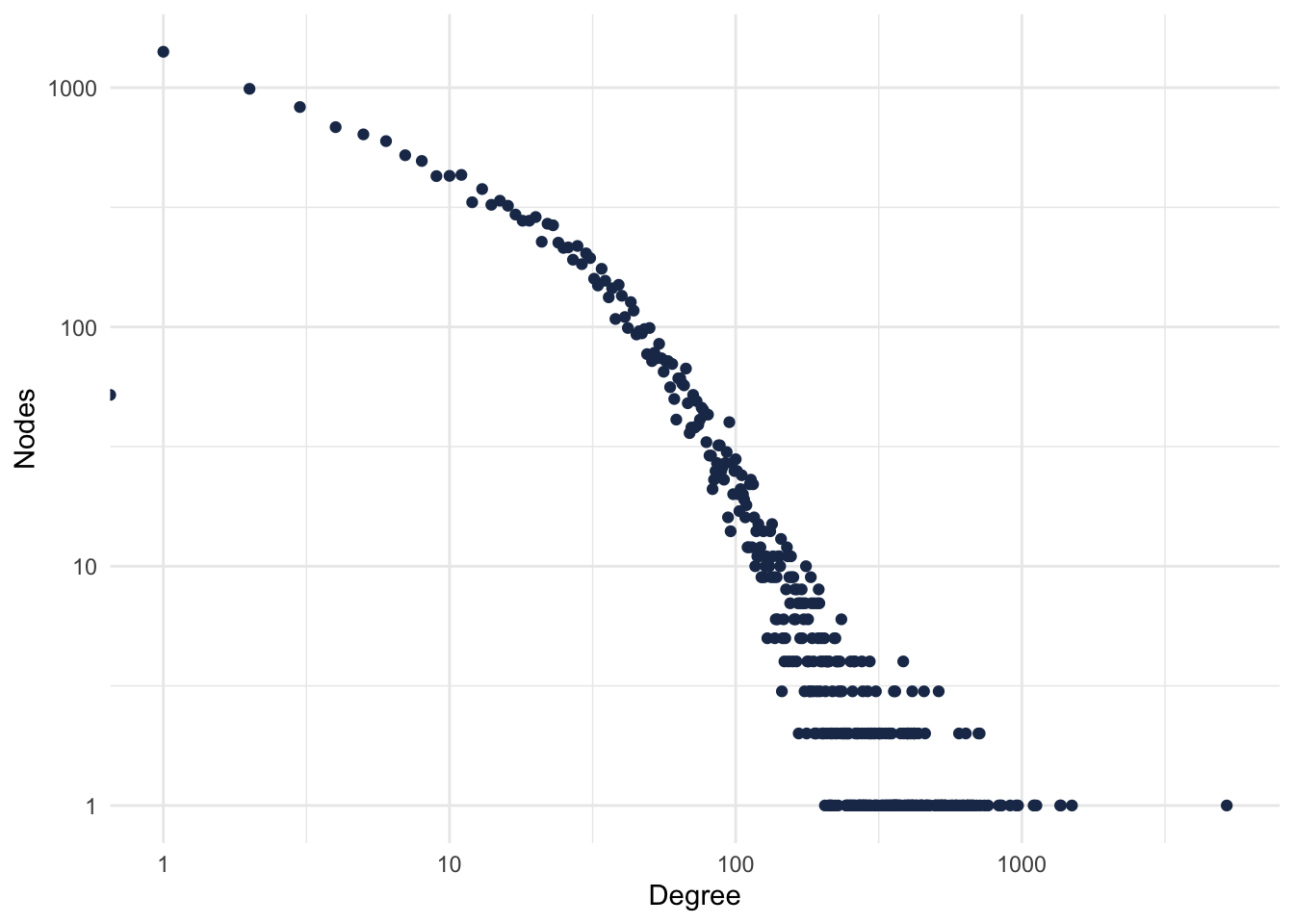
Figure 1: PPI Degree Distribution.
Most of the proteins have few connections, and very few proteins have lots of connections. Who’s that protein?
##          .
## UBC   5199
## ETS1  1496
## GATA2 1369
## CTCF  1361
## EP300 1124
## MYC   1107
## AR    1099
Exercises
Now is your turn. Spend some minutes understanding the data and getting some familiarity with it.
What are the top 10 genes with the highest degree?
Are those genes connected?
## IGRAPH 685f946 UN-- 10 24 --
## + attr: name (v/c)
## + edges from 685f946 (vertex names):
##  [1] MYC  --CTCF  EGR1 --ETS1  EGR1 --EP300 MYC  --EP300 ETS1 --EP300
##  [6] EGR1 --UBC   MYC  --UBC   CTCF --UBC   ETS1 --UBC   EP300--UBC
## [11] EGR1 --AR    MYC  --AR    ETS1 --AR    EP300--AR    UBC  --AR
## [16] EGR1 --GATA2 MYC  --GATA2 ETS1 --GATA2 EP300--GATA2 CTCF --APP
## [21] UBC  --APP   MYC  --RAD21 CTCF --RAD21 UBC  --RAD21
Gene Disease Association
A Gene-Disease-Association (GDA) database are typically used to understand the association of genes to diseases, and model the underlying mechanisms of complex diseases. Those associations often come from GWAS studies and knock-out studies.
Commonly used data sources for GDAs
As PPIs, GDAs can be found from different sources and with different evidences for each Gene-Disease association. I list here some well-known databases for that.
CTD – Curated scientific literature (Davis et al. 2020)
OMIM – Curated scientific literature (McKusick 2007)
DisGeNet – Based on OMIM, ClinVar, and other data bases (Piñero et al. 2019)
Orphanet – Validated - and non-validated - GDAs
ClinGen – Validated - and non-validated - GDAs (Rehm et al. 2015)
ClinVar – Different levels of evidence (Landrum et al. 2019)
GWAS catalogue – GWAS associations to diseases (Buniello et al. 2018)
PheGenI – GWAS associations to diseases (Ramos et al. 2013)
lncRNADisease – Experimentally validated lncRNAs in diseases (Chen et al. 2012)
HMDD – Experimentally validated miRNAs in diseases (Huang et al. 2018)
Understanding a GDA dataset
We will use in this workshop Gene-Disease-Association from DisGeNet. It can be found here.
Similar to the PPI, let us first get some familiarity with the data, before performing any analysis.
Let’s read in the data and, again, do some basic statistics.
GDA = fread(file = './data/curated_gene_disease_associations.tsv', sep = '\t')

head(GDA)
## geneId geneSymbol DSI DPI diseaseId diseaseName diseaseType
## 1: 1 A1BG 0.700 0.538 C0019209 Hepatomegaly phenotype
## 2: 1 A1BG 0.700 0.538 C0036341 Schizophrenia disease
## 3: 2 A2M 0.529 0.769 C0002395 Alzheimer's Disease disease
## 4: 2 A2M 0.529 0.769 C0007102 Malignant tumor of colon disease
## 5: 2 A2M 0.529 0.769 C0009375 Colonic Neoplasms group
## 6: 2 A2M 0.529 0.769 C0011265 Presenile dementia disease
## diseaseClass diseaseSemanticType score EI YearInitial
## 1: C23;C06 Finding 0.30 1.000 2017
## 2: F03 Mental or Behavioral Dysfunction 0.30 1.000 2015
## 3: C10;F03 Disease or Syndrome 0.50 0.769 1998
## 4: C06;C04 Neoplastic Process 0.31 1.000 2004
## 5: C06;C04 Neoplastic Process 0.30 1.000 2004
## 6: C10;F03 Mental or Behavioral Dysfunction 0.30 1.000 1998
## YearFinal NofPmids NofSnps source
## 1: 2017 1 0 CTD_human
## 2: 2015 1 0 CTD_human
## 3: 2018 3 0 CTD_human
## 4: 2019 1 0 CTD_human
## 5: 2004 1 0 CTD_human
## 6: 2004 3 0 CTD_humanThe first thing to notice is the inconsistency with the disease names, in order to be able to work with it, let’s first put every disease to lower-case.
Let’s also understand the degree distribution of the diseases.
numGenes = Cleaned_GDA %>%
  group_by(diseaseName) %>%
  summarise(numGenes = n()) %>%
  ungroup() %>%
  group_by(numGenes) %>%
  summarise(numDiseases = n())
numGenes = Cleaned_GDA %>%
group_by(diseaseName) %>%
summarise(numGenes = n()) %>%
ungroup() %>%
group_by(numGenes) %>%
summarise(numDiseases = n())
ggplot(numGenes) +
aes(x = numGenes, y = numDiseases) +
geom_point(colour = "#1d3557") +
scale_x_continuous(trans = "log10") +
scale_y_continuous(trans = "log10") +
labs(x = "Genes", y = "Diseases")+
theme_minimal()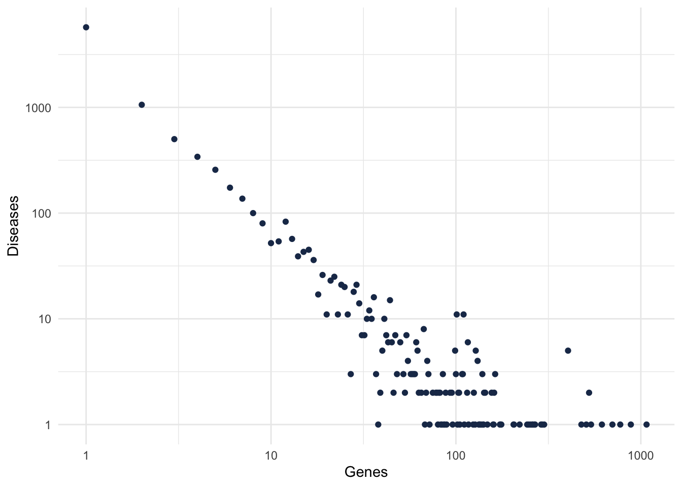
Figure 2: Gene-Disease degree distribution.
Because we want to focus in well studied diseases, and also that are known to be complex diseases, let’s filter for diseases with at least 10 genes.
Cleaned_GDA %<>%
  group_by(diseaseName) %>%
  mutate(numGenes = n()) %>%
  filter(numGenes > 10)

Cleaned_GDA$diseaseName %>%
  unique() %>%
  length()
## [1] 920Exercises
Now is your turn. Spend some minutes understanding the data and getting some familiarity with it.
- What are the top 10 genes mostly involved with diseases? What are those diseases?
## # A tibble: 10 x 3
##    geneSymbol numDis index
##    <chr>       <int> <int>
##  1 TNF           177     1
##  2 IL6           144     2
##  3 SOD2          144     3
##  4 TP53          138     4
##  5 PTGS2         128     5
##  6 MTHFR         117     6
##  7 IL1B          115     7
##  8 PTEN          105     8
##  9 TGFB1         105     9
## 10 KRAS 100 10- What are the top 10 highly polygenic diseases?
## # A tibble: 10 x 3
##    diseaseName                    numGenes index
##    <chr>                             <int> <int>
##  1 malignant neoplasm of breast       1074     1
##  2 schizophrenia                       883     2
##  3 liver cirrhosis, experimental       774     3
##  4 colorectal carcinoma                702     4
##  5 malignant neoplasm of prostate      616     5
##  6 breast carcinoma                    538     6
##  7 mammary carcinoma, human            525     7
##  8 mammary neoplasms, human            525     8
##  9 liver carcinoma                     507     9
## 10 bipolar disorder 477 10- What are the top 10 highly polygenic disease classes?
## # A tibble: 10 x 3
##    diseaseSemanticType                               numGenes index
##    <chr>                                                <int> <int>
##  1 Disease or Syndrome                                  18033     1
##  2 Neoplastic Process                                   16163     2
##  3 Mental or Behavioral Dysfunction                      6015     3
##  4 Congenital Abnormality                                1325     4
##  5 Experimental Model of Disease                         1300     5
##  6 Injury or Poisoning                                   1027     6
##  7 Neoplastic Process; Experimental Model of Disease      330     7
##  8 Acquired Abnormality                                   106     8
##  9 Pathologic Function                                     72     9
## 10 Disease or Syndrome; Congenital Abnormality             68    10
Methods for Disease Module Identification and Disease Similarity
In this chapter, I will introduce the main methods used in Network Medicine. We will start by understanding what a Disease Module is, how we can calculate its significance, and also understand its importance. Next, we will explore the disease separation, how to calculate, and make interpretations.
Disease Module
In biological networks, genes are often involved in the same topological communities are also associated with similar biological processes (Ahn, Bagrow, and Lehmann 2010). It also reflects on how diseases localized themselves in the interaction; meaning that, disease modules are highly localized in specific network neighborhoods (Menche et al. 2015).
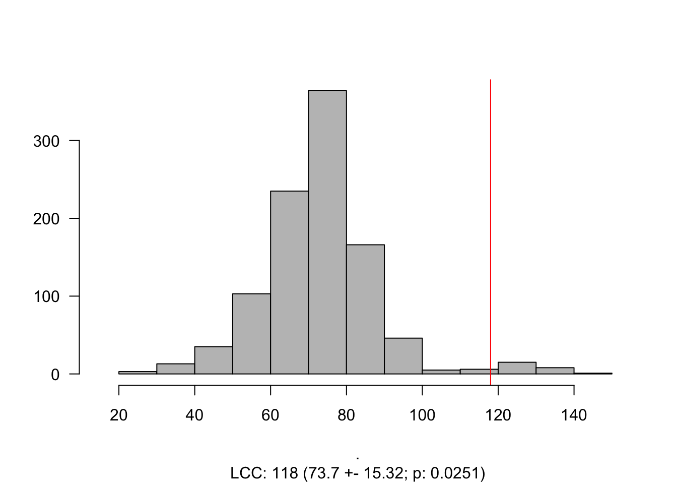
Largest connected component
The size of the largest connected component (LCC) is the number of nodes that form a connected subgraph (in our case, it is the number of proteins that are interconnected in the PPI). Many properties of this quantity allow us to understand how a particular disease interacts with the interactome. It is important to note here that this measure is highly dependent on the completeness of an interactome. If a link between a protein and its counterparts is unknown – therefore missing – we might say that that particular node is not involved in a disease module (or that the LCC is not significant).
Figure 3: Disease-Module. In a schematic of a PPI, in pink, we see genes associated with a disease, forming a connected component of size 4.
However, just computing this number might not be informative, and it is expected a randomness. To calculate this randomness, we often calculate the significance of the LCC by selecting proteins in the interactome with similar degrees (aka degree preserving randomization).
To calculate the significance of the LCC, one can calculate its Z-Score or simply calculate the empirical probability under the curve from the empirical distribution. The Z-score is given by:
\[ Z-Score_{LCC} = \frac{LCC - \mu_{LCC}}{\sigma_{LCC}}. \]
Example in real data
Our first task now is to understand if some diseases, from our Cleaned_GDA are able to form a Disease-Module. Let’s start doing it for Schizophrenia and later we will add some more diseases.
The idea now is: Gather the genes associated to our disease in the data, find them in the PPI, check if they form a connected component, check the significance of the component and visualize the Disease-Module.
# First, let's attach all packages we will need.
require(NetSci)
require(magrittr)
require(dplyr)
require(igraph)
#First, let's select genes that are associated with Schizophrenia.
SCZ_Genes =
Cleaned_GDA %>%
filter(diseaseName %in% 'schizophrenia') %>%
pull(geneSymbol) %>%
unique()
# Next, let's see how they are localized in the PPI.
# Fist, we have to make sure all genes are in the PPI.
# Later, we calculate the LCC.
# And lastly, let's visualize it.
SCZ_PPI = SCZ_Genes[SCZ_Genes %in% V(gPPI)$name]
gScz = gPPI %>%
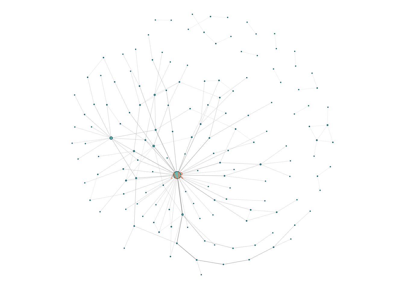
induced.subgraph(., SCZ_PPI)components(gScz)$csize %>% max## [1] 683The size of the LCC is 683. However, how does it compare to a random selection genes?
LCC_scz = LCC_Significance(N = 100,
                           Targets = SCZ_PPI,
                           G = gPPI)
Histogram_LCC(LCC_scz)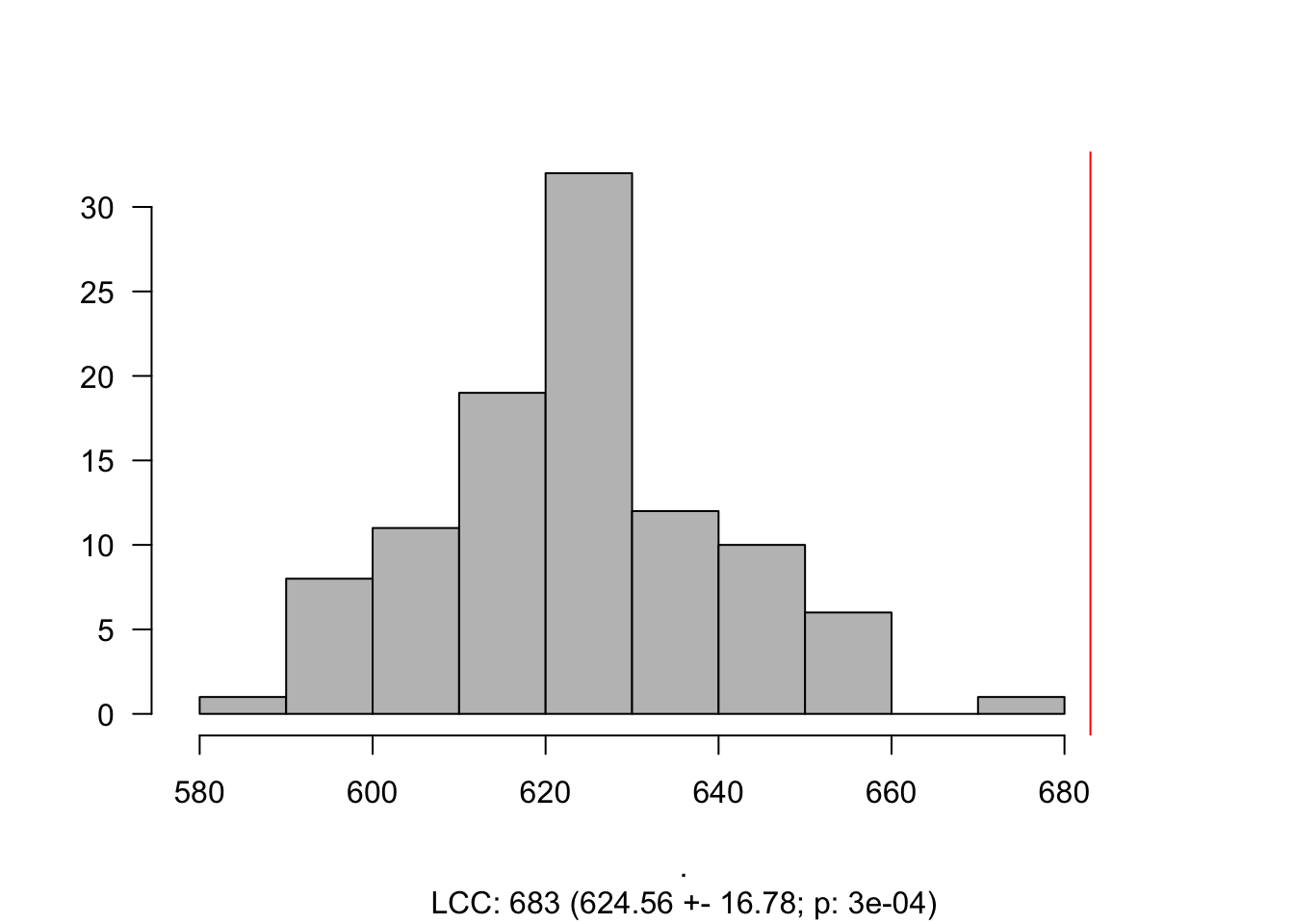
gScz ## IGRAPH 3f9cbf3 UN-- 846 2564 --
## + attr: name (v/c)
## + edges from 3f9cbf3 (vertex names):
## [1] PI4KA --SP1 F2 --SP1 DNM1 --CTCF GSK3B --HSPA1A
## [5] DNM1 --GRB2 SP1 --GRB2 MET --GRB2 GSK3B --MAPK14
## [9] SP1 --MAPK14 CTCF --MAPK14 GRB2 --MAPK14 MET --ACTB
## [13] GRB2 --ACTB MAPK14 --ACTB GSK3B --SOX10 SP1 --SOX10
## [17] PAX6 --SOX10 SP1 --CCNA2 ACTB --MTNR1A ACTB --GSN
## [21] PI4KA --JUN GSK3B --JUN SMARCA2--JUN SP1 --JUN
## [25] MAPK14 --JUN SOX10 --JUN GSK3B --ESR1 SMARCA2--ESR1
## [29] SP1 --ESR1 HSPA1A --ESR1 FMR1 --ESR1 MAPK14 --ESR1
## + ... omitted several edgesV(gScz)$size = degree(gScz) %>%
CoDiNA::normalize()
V(gScz)$size = (V(gScz)$size + 0.1)*5
V(gScz)$color = '#83c5be'
V(gScz)$frame.color = '#006d77'
V(gScz)$label = ifelse(V(gScz)$size > 4, V(gScz)$name, NA )
V(gScz)$label.color = '#e29578'
E(gScz)$width = edge.betweenness(gScz, directed = F) %>% CoDiNA::normalize()
E(gScz)$width = E(gScz)$width + 0.01
E(gScz)$weight = E(gScz)$width
par(mar = c(0,0,0,0))
plot(gScz)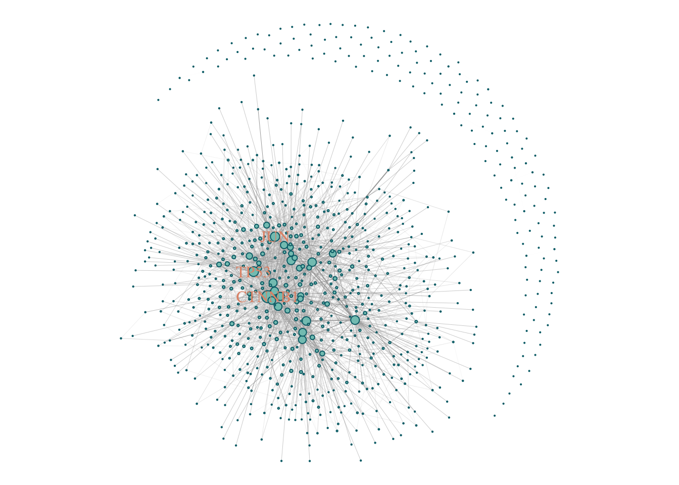
Let’s remove all genes with degree = 0. (Genes that do not connect to any other gene).
gScz %<>% delete.vertices(., degree(.) == 0)
V(gScz)$size = degree(gScz) %>%
  CoDiNA::normalize()
V(gScz)$size = (V(gScz)$size + 0.1)*5
V(gScz)$color = '#83c5be'
V(gScz)$frame.color = '#006d77'
V(gScz)$label = ifelse(V(gScz)$size  > 4, V(gScz)$name, NA )
V(gScz)$label.color = '#e29578'

E(gScz)$width = edge.betweenness(gScz, directed = F) %>% CoDiNA::normalize()
E(gScz)$width = E(gScz)$width + 0.01
E(gScz)$weight = E(gScz)$width
par(mar = c(0,0,0,0))
plot(gScz)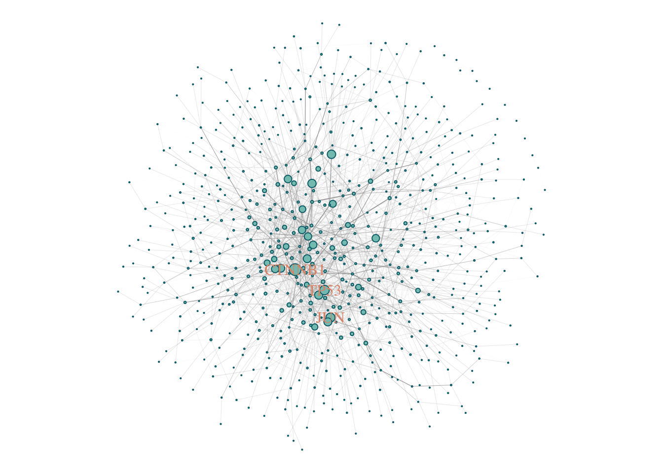
Exercises
- Calculate the LCC, and visualize the modules for the following diseases:
- Autistic Disorder;
Bipolar Disorder;
Major Depressive Disorder;
Rheumatoid Arthritis;
Asthma
Parkinson Disease
Endometriosis
Gene Overlap
A first intuitive way to measure the overlap of two gene sets is by calculating its overlap, or its normalized overlap, the Jaccard Index. The Jaccard index is calculated by taking the ratio of Intersection of two sets over the Union of those sets. The Jaccard coefficient measures similarity between finite sample sets, and is defined as the size of the intersection divided by the size of the union of the sample sets:
\[ J(A,B) = \frac{|A \cap B|}{|A \cup B|} = \frac{|A \cap B|}{|A| + |B| - |A \cap B|}. \]
Note that by design, \(0 \leq J(A,B) \leq 1\). If A and B are both empty, define \(J(A,B) = 1\).
Let’s calculate the Jaccard Index for the diseases we calculated its LCCs.
Dis_Ex1 = c('schizophrenia',
            'autistic disorder',
            'bipolar disorder',
            "major depressive disorder",
            'asthma',
            'rheumatoid arthritis',
            'parkinson disease',
            'endometriosis')
GDA_Interest = Cleaned_GDA %>%
  filter(diseaseName %in% Dis_Ex1) %>%
  select(diseaseName, geneSymbol) %>%
  unique()

Jaccard_Ex2 = Jaccard(GDA_Interest)
##
|
| | 0%
|
|========= | 12%
|
|================== | 25%
|
|========================== | 38%
|
|=================================== | 50%
|
|============================================ | 62%
|
|==================================================== | 75%
|
|============================================================= | 88%
|
|======================================================================| 100%Jaccard_Ex2## Node.1 Node.2 Jaccard.Index
## 1: schizophrenia autistic disorder 0.09578544
## 2: schizophrenia bipolar disorder 0.21428571
## 3: autistic disorder bipolar disorder 0.09658247
## 4: schizophrenia major depressive disorder 0.11817279
## 5: autistic disorder major depressive disorder 0.08154506
## 6: bipolar disorder major depressive disorder 0.16316640
## 7: schizophrenia endometriosis 0.01655307
## 8: autistic disorder endometriosis 0.02676399
## 9: bipolar disorder endometriosis 0.02243590
## 10: major depressive disorder endometriosis 0.03589744
## 11: schizophrenia parkinson disease 0.03308431
## 12: autistic disorder parkinson disease 0.03903904
## 13: bipolar disorder parkinson disease 0.03690037
## 14: major depressive disorder parkinson disease 0.06493506
## 15: endometriosis parkinson disease 0.01652893
## 16: schizophrenia asthma 0.02337938
## 17: autistic disorder asthma 0.04281346
## 18: bipolar disorder asthma 0.03148148
## 19: major depressive disorder asthma 0.02866242
## 20: endometriosis asthma 0.02118644
## 21: parkinson disease asthma 0.05095541
## 22: schizophrenia rheumatoid arthritis 0.02721088
## 23: autistic disorder rheumatoid arthritis 0.03571429
## 24: bipolar disorder rheumatoid arthritis 0.03169572
## 25: major depressive disorder rheumatoid arthritis 0.04511278
## 26: endometriosis rheumatoid arthritis 0.02446483
## 27: parkinson disease rheumatoid arthritis 0.02777778
## 28: asthma rheumatoid arthritis 0.04958678
## Node.1 Node.2 Jaccard.Index# Let's visualize the Venn diagram (Euler Diagram) of those overlaps.
require(eulerr)## Loading required package: eulerrEuler_List = list (
SCZ = GDA_Interest$geneSymbol[GDA_Interest$diseaseName == 'schizophrenia'],
ASD = GDA_Interest$geneSymbol[GDA_Interest$diseaseName == 'autistic disorder'],
BD = GDA_Interest$geneSymbol[GDA_Interest$diseaseName == 'bipolar disorder'],
MDD = GDA_Interest$geneSymbol[GDA_Interest$diseaseName == 'major depressive disorder'],
AT = GDA_Interest$geneSymbol[GDA_Interest$diseaseName == 'asthma'],
RA = GDA_Interest$geneSymbol[GDA_Interest$diseaseName == 'rheumatoid arthritis'],
ED = GDA_Interest$geneSymbol[GDA_Interest$diseaseName == 'endometriosis'],
PD = GDA_Interest$geneSymbol[GDA_Interest$diseaseName == 'parkinson disease'])
EULER = euler(Euler_List)
plot(EULER, quantities = TRUE)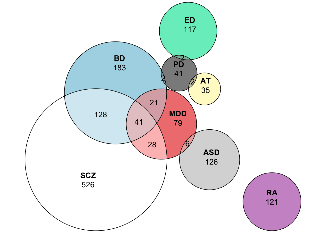
Disease Separation
When looking into the Jaccard Index, we have a sense of how similar two diseases are based on genes that are known to be associated with both diseases. The main problem with this is that we assume that all genes associated with a disease is known, and we do not take the topology of the underlying network into account.
The separation is a complementary quantity that is a bit less sensitive to the incompleteness of the PPI, we can measure the distances \(d_s\) of each disease-associated node to all other disease associated nodes. Taking into account only the shortest distance between them results in a distribution \(P(d_s)\). The mean value \(<d_s>\) can be interpreted as the diameter of the disease model. Note the diameter here is the average distance instead of the maximal distance.
The concept of network localization can be further generalized to examine the relationship between any different sets of nodes, for example, proteins associated with two different diseases. The network serves as a map, where diseases are represented by different neighborhoods. How close and the degree of overlap of two network neighborhoods can be found to be highly predictive of the pathological similarity of those diseases (Menche et al. 2015).
To quantify the distance of two sets of nodes A and B, we first compute the distribution \(P(d_{AB})\) of all shortest distances \(d_{AB}\) between nodes A and B and the respective mean distance \(<d_{AB}>\).
The network based separation \(S_{AB}\) can be obtained by comparing the mean shortest distance within the respective node sets and the mean shortest distance between them.
\[ S_{AB} = <d_{AB}> - \frac{<d_{AA}> + <d_BB>}{2}. \]
Note: negative \(S_{AB}\) indicates topological overlap of the two node sets, while a positive \(S_{AB}\) indicates a topological separation of the two node sets.
The size of the overlap is highly predictive of pathological and functional similarity, elevated co-expression, symptoms similarity, and high comorbidity diseases.
Figure 4: Disease-Separation. In a schematic PPI, we see genes associated with a disease A (in pink), and genes associated to disease B (in green).
The separation of diseases A and B is given by: \[ <d_{AA}> = 1.5 \]
\[ <d_{BB}> = 1.5 \]
\[ <d_{AB}> = 2.7 \] \[ S_{AB} = 2.7 - \frac{1.5+ 1.5}2 = 1.2. \]
Example in real data
sab = separation(gPPI, GDA_Interest)##
|
| | 0%
|
|========= | 12%
|
|================== | 25%
|
|========================== | 38%
|
|=================================== | 50%
|
|============================================ | 62%
|
|==================================================== | 75%
|
|============================================================= | 88%
|
|======================================================================| 100%## Calculating S_ab..##
|
| | 0%
|
|========= | 12%
|
|================== | 25%
|
|========================== | 38%
|
|=================================== | 50%
|
|============================================ | 62%
|
|==================================================== | 75%
|
|============================================================= | 88%
|
|======================================================================| 100%## Done..sab## $Sab
## schizophrenia autistic disorder bipolar disorder
## schizophrenia 0 -0.1045849 -0.4157872
## autistic disorder NA 0.0000000 -0.1548042
## bipolar disorder NA NA 0.0000000
## major depressive disorder NA NA NA
## endometriosis NA NA NA
## parkinson disease NA NA NA
## asthma NA NA NA
## rheumatoid arthritis NA NA NA
## major depressive disorder endometriosis
## schizophrenia -0.1340951 0.22202922
## autistic disorder -0.1132453 0.09132126
## bipolar disorder -0.2881742 0.16886859
## major depressive disorder 0.0000000 0.05226307
## endometriosis NA 0.00000000
## parkinson disease NA NA
## asthma NA NA
## rheumatoid arthritis NA NA
## parkinson disease asthma rheumatoid arthritis
## schizophrenia 0.25050220 0.27686802 0.17548173
## autistic disorder 0.05937602 0.07992430 0.04855410
## bipolar disorder 0.18588070 0.17716612 0.12075995
## major depressive disorder 0.04371349 0.14222353 0.02800574
## endometriosis 0.14567472 0.06544036 0.02120766
## parkinson disease 0.00000000 0.03649188 0.11030856
## asthma NA 0.00000000 0.01226364
## rheumatoid arthritis NA NA 0.00000000
##
## $Dab
## schizophrenia autistic disorder bipolar disorder
## schizophrenia 1.176331 1.185962 0.8217292
## autistic disorder NA 1.404762 1.1969274
## bipolar disorder NA NA 1.2987013
## major depressive disorder NA NA NA
## endometriosis NA NA NA
## parkinson disease NA NA NA
## asthma NA NA NA
## rheumatoid arthritis NA NA NA
## major depressive disorder endometriosis
## schizophrenia 1.120037 1.529940
## autistic disorder 1.255102 1.513447
## bipolar disorder 1.027143 1.537964
## major depressive disorder 1.331933 1.437975
## endometriosis NA 1.439490
## parkinson disease NA NA
## asthma NA NA
## rheumatoid arthritis NA NA
## parkinson disease asthma rheumatoid arthritis
## schizophrenia 1.600863 1.668831 1.483301
## autistic disorder 1.523952 1.586103 1.470588
## bipolar disorder 1.597426 1.630314 1.489764
## major depressive disorder 1.471875 1.611987 1.413625
## endometriosis 1.627615 1.588983 1.460606
## parkinson disease 1.524390 1.602484 1.592157
## asthma NA 1.607595 1.535714
## rheumatoid arthritis NA NA 1.439306Sep_ex2 = sab$Sab %>% as.matrix()
Sep_ex2[lower.tri(Sep_ex2)] = t(Sep_ex2)[lower.tri(Sep_ex2)]We can visualize the network separation of the diseases using a heatmap.
Sep_ex2 %>% heatmap(., symm = T)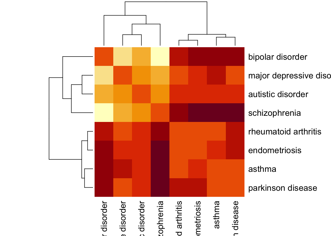
Exercises
- Calculate the Jaccard Index and the Separation for the diseases that have
diseaseSemanticTypeas Mental or Behavioral Dysfunction.
##
  |
  |                                                                      |   0%
  |
  |=                                                                     |   1%
  |
  |==                                                                    |   3%
  |
  |===                                                                   |   4%
  |
  |====                                                                  |   6%
  |
  |=====                                                                 |   7%
  |
  |======                                                                |   8%
  |
  |=======                                                               |  10%
  |
  |========                                                              |  11%
  |
  |=========                                                             |  13%
  |
  |==========                                                            |  14%
  |
  |===========                                                           |  15%
  |
  |============                                                          |  17%
  |
  |=============                                                         |  18%
  |
  |==============                                                        |  20%
  |
  |===============                                                       |  21%
  |
  |================                                                      |  23%
  |
  |=================                                                     |  24%
  |
  |==================                                                    |  25%
  |
  |===================                                                   |  27%
  |
  |====================                                                  |  28%
  |
  |=====================                                                 |  30%
  |
  |======================                                                |  31%
  |
  |=======================                                               |  32%
  |
  |========================                                              |  34%
  |
  |=========================                                             |  35%
  |
  |==========================                                            |  37%
  |
  |===========================                                           |  38%
  |
  |============================                                          |  39%
  |
  |=============================                                         |  41%
  |
  |==============================                                        |  42%
  |
  |===============================                                       |  44%
  |
  |================================                                      |  45%
  |
  |=================================                                     |  46%
  |
  |==================================                                    |  48%
  |
  |===================================                                   |  49%
  |
  |===================================                                   |  51%
  |
  |====================================                                  |  52%
  |
  |=====================================                                 |  54%
  |
  |======================================                                |  55%
  |
  |=======================================                               |  56%
  |
  |========================================                              |  58%
  |
  |=========================================                             |  59%
  |
  |==========================================                            |  61%
  |
  |===========================================                           |  62%
  |
  |============================================                          |  63%
  |
  |=============================================                         |  65%
  |
  |==============================================                        |  66%
  |
  |===============================================                       |  68%
  |
  |================================================                      |  69%
  |
  |=================================================                     |  70%
  |
  |==================================================                    |  72%
  |
  |===================================================                   |  73%
  |
  |====================================================                  |  75%
  |
  |=====================================================                 |  76%
  |
  |======================================================                |  77%
  |
  |=======================================================               |  79%
  |
  |========================================================              |  80%
  |
  |=========================================================             |  82%
  |
  |==========================================================            |  83%
  |
  |===========================================================           |  85%
  |
  |============================================================          |  86%
  |
  |=============================================================         |  87%
  |
  |==============================================================        |  89%
  |
  |===============================================================       |  90%
  |
  |================================================================      |  92%
  |
  |=================================================================     |  93%
  |
  |==================================================================    |  94%
  |
  |===================================================================   |  96%
  |
  |====================================================================  |  97%
  |
  |===================================================================== |  99%
  |
  |======================================================================| 100%
## Calculating S_ab..##
|
| | 0%
|
|= | 1%
|
|== | 3%
|
|=== | 4%
|
|==== | 6%
|
|===== | 7%
|
|====== | 8%
|
|======= | 10%
|
|======== | 11%
|
|========= | 13%
|
|========== | 14%
|
|=========== | 15%
|
|============ | 17%
|
|============= | 18%
|
|============== | 20%
|
|=============== | 21%
|
|================ | 23%
|
|================= | 24%
|
|================== | 25%
|
|=================== | 27%
|
|==================== | 28%
|
|===================== | 30%
|
|====================== | 31%
|
|======================= | 32%
|
|======================== | 34%
|
|========================= | 35%
|
|========================== | 37%
|
|=========================== | 38%
|
|============================ | 39%
|
|============================= | 41%
|
|============================== | 42%
|
|=============================== | 44%
|
|================================ | 45%
|
|================================= | 46%
|
|================================== | 48%
|
|=================================== | 49%
|
|=================================== | 51%
|
|==================================== | 52%
|
|===================================== | 54%
|
|====================================== | 55%
|
|======================================= | 56%
|
|======================================== | 58%
|
|========================================= | 59%
|
|========================================== | 61%
|
|=========================================== | 62%
|
|============================================ | 63%
|
|============================================= | 65%
|
|============================================== | 66%
|
|=============================================== | 68%
|
|================================================ | 69%
|
|================================================= | 70%
|
|================================================== | 72%
|
|=================================================== | 73%
|
|==================================================== | 75%
|
|===================================================== | 76%
|
|====================================================== | 77%
|
|======================================================= | 79%
|
|======================================================== | 80%
|
|========================================================= | 82%
|
|========================================================== | 83%
|
|=========================================================== | 85%
|
|============================================================ | 86%
|
|============================================================= | 87%
|
|============================================================== | 89%
|
|=============================================================== | 90%
|
|================================================================ | 92%
|
|================================================================= | 93%
|
|================================================================== | 94%
|
|=================================================================== | 96%
|
|==================================================================== | 97%
|
|===================================================================== | 99%
|
|======================================================================| 100%## Done..##
|
| | 0%
|
|= | 1%
|
|== | 3%
|
|=== | 4%
|
|==== | 6%
|
|===== | 7%
|
|====== | 8%
|
|======= | 10%
|
|======== | 11%
|
|========= | 13%
|
|========== | 14%
|
|=========== | 15%
|
|============ | 17%
|
|============= | 18%
|
|============== | 20%
|
|=============== | 21%
|
|================ | 23%
|
|================= | 24%
|
|================== | 25%
|
|=================== | 27%
|
|==================== | 28%
|
|===================== | 30%
|
|====================== | 31%
|
|======================= | 32%
|
|======================== | 34%
|
|========================= | 35%
|
|========================== | 37%
|
|=========================== | 38%
|
|============================ | 39%
|
|============================= | 41%
|
|============================== | 42%
|
|=============================== | 44%
|
|================================ | 45%
|
|================================= | 46%
|
|================================== | 48%
|
|=================================== | 49%
|
|=================================== | 51%
|
|==================================== | 52%
|
|===================================== | 54%
|
|====================================== | 55%
|
|======================================= | 56%
|
|======================================== | 58%
|
|========================================= | 59%
|
|========================================== | 61%
|
|=========================================== | 62%
|
|============================================ | 63%
|
|============================================= | 65%
|
|============================================== | 66%
|
|=============================================== | 68%
|
|================================================ | 69%
|
|================================================= | 70%
|
|================================================== | 72%
|
|=================================================== | 73%
|
|==================================================== | 75%
|
|===================================================== | 76%
|
|====================================================== | 77%
|
|======================================================= | 79%
|
|======================================================== | 80%
|
|========================================================= | 82%
|
|========================================================== | 83%
|
|=========================================================== | 85%
|
|============================================================ | 86%
|
|============================================================= | 87%
|
|============================================================== | 89%
|
|=============================================================== | 90%
|
|================================================================ | 92%
|
|================================================================= | 93%
|
|================================================================== | 94%
|
|=================================================================== | 96%
|
|==================================================================== | 97%
|
|===================================================================== | 99%
|
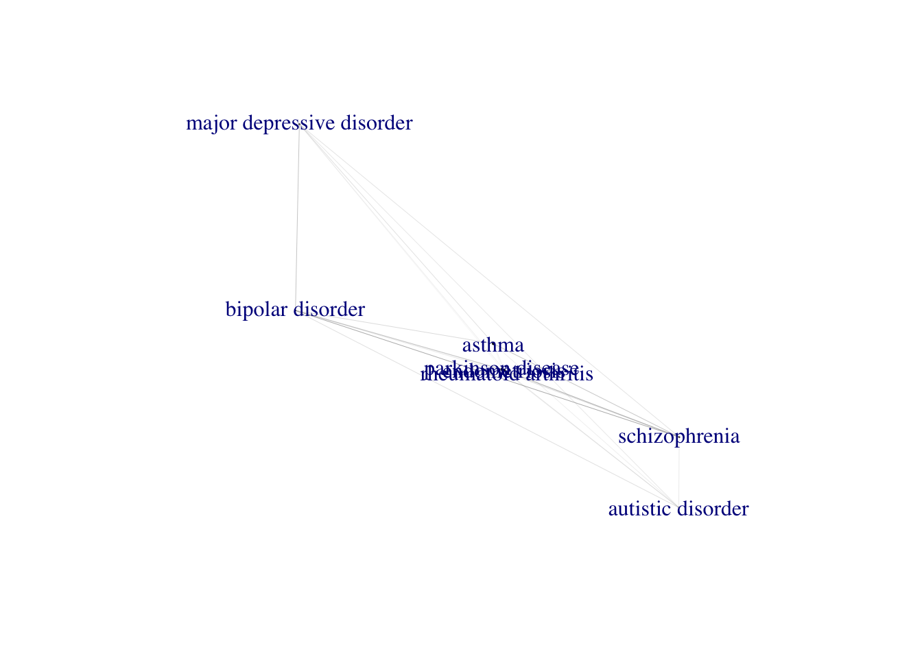
|======================================================================| 100%- Optional: Try to make the network visualization for the heatmap of
Sep_ex2. Use diseases as nodes, and their weight as links.
- Optional: If we go back to our PPI, can we identify that the modules are indeed close or separated? Plot the network for those diseases.
Gene Co-expression Networks
In co-expression networks, a pair of nodes is typically connected by a link if the genes they represent show a significantly correlated expression pattern across a set of biological samples of interest. They are often built from genome-wide expression data measured by RNA-Seq or microarrays. Those networks are often weighted, and it represents the strength of a gene-pair relationship. Gene co-expression networks are also signed, and the sign of the link can be indicative of whether a gene pair is regulated in the same direction or oppositely controlled. The majority of the methods used for constructing those networks rely on a similarity measure, such as mutual information or correlation. In this course, we will use the wTO (Deisy Morselli Gysi et al. 2018; Nowick et al. 2009) method . This is a correlation based method, that normalizes the effect of the interaction by all gene neibours and that also accounts for positive and negative interactions. It also calculates the probability for each gene pair, reducing the false positive links.
A next step for co-expression analysis is by comparing the resulting networks for different groups. For that the CoDiNA (Co-expression Differential Network Analysis) (Morselli Gysi et al. 2020) method can be used.
Construction of co-expression networks
To run the weighted topological overlap (wTO) in R we can easily do by loading the wTO R package. It calculates the networks using expression data, where genes are on the rows and individuals in the columns. The user can select parallel computing for faster computation.
For the sake of time, we will be focusing here on the network of differential expressed genes. However, in a real set-up, the best approach is to use the full set of genes.
For the analysis we will be using the data from GSE12654 (Iwamoto et al. 2004). The file here contains Pre Frontal Cortex samples from Control and patients with Bipolar Disorder, Schizophrenia and Major Depression, and is already filtered for only differential expressed genes.
- Let’s read in the data:
require(wTO)## Loading required package: wTOrequire(CoDiNA)## Loading required package: CoDiNA##
## Attaching package: 'CoDiNA'## The following objects are masked from 'package:igraph':
##
## as.igraph, normalizeBrain = fread("./data/Brain.csv") %>%
as.data.frame()
row.names(Brain) = Brain$V1
Brain = Brain[,-1]- Let’s look into it:
##          BD_ID1   BD_ID2   BD_ID3   BD_ID4   BD_ID5   BD_ID6   BD_ID7   BD_ID8
## HSF1   7.593522 7.414498 7.551313 7.604576 7.818765 7.452378 7.505604 7.570283
## PDLIM5 4.194690 4.300449 4.141026 4.067548 4.296824 4.309824 4.394849 4.166770
## MSX2   3.912240 3.841050 3.701938 3.912098 3.703137 3.700736 3.969032 3.650190
## PML    6.565121 6.569837 6.551878 6.570909 6.629373 6.553288 6.677511 6.553654
## DEDD   6.043961 5.914945 6.169624 5.811971 5.874334 6.040275 5.941909 6.045629
## RAB8A  6.235237 6.353685 6.318565 6.209181 6.272028 6.468419 6.246321 6.351017
## ELF3   4.879226 4.481001 4.630118 4.943885 4.642466 4.624869 4.515094 4.670392
## CDC5L  2.918337 2.742434 2.814158 2.760304 2.870200 2.748367 2.831504 2.768490
## ZNF211 4.448121 4.722869 4.285932 4.690489 4.267327 4.328995 4.376896 4.396760
## FOXF2  4.525340 4.818690 4.936654 4.772364 4.921325 4.825912 5.031065 4.687238
##          BD_ID9  BD_ID10
## HSF1   7.905238 7.704259
## PDLIM5 4.649225 3.909871
## MSX2   3.896163 3.918197
## PML    6.480951 6.526635
## DEDD   6.093379 6.216374
## RAB8A  6.258136 6.637794
## ELF3   4.605525 4.488687
## CDC5L  2.861687 2.910959
## ZNF211 4.793549 4.824614
## FOXF2 4.923211 4.978635- How to run the
wTO?
You’ll need a data.frame with genes on the rows, individuals on the columns, gene names on the row.names. We also need to create one network per disease.
BD = Brain %>%
  dplyr::select(starts_with('BD')) %>%
  wTO.fast(n = 100, Data = .)
## There are 198 overlapping nodes, 198 total nodes and 11 individuals.## This function might take a long time to run. Don't turn off the computer.## 1 2 3 4 5 6 7 8 9 10 11 12 13 14 15 16 17 18 19 20 21 22 23 24 25 26 27 28 29 30 31 32 33 34 35 36 37 38 39 40 41 42 43 44 45 46 47 48 49 50 51 52 53 54 55 56 57 58 59 60 61 62 63 64 65 66 67 68 69 70 71 72 73 74 75 76 77 78 79 80 81 82 83 84 85 86 87 88 89 90 91 92 93 94 95 96 97 98 99 100 Done!- Let’s explore the output
##    Node.1 Node.2    wTO pval  pval.adj
## 1:   HSF1 PDLIM5  0.221 0.56 0.5885160
## 2:   HSF1   MSX2  0.112 0.34 0.5780850
## 3: PDLIM5   MSX2 -0.076 0.46 0.5780850
## 4:   HSF1    PML -0.150 0.48 0.5780850
## 5: PDLIM5    PML  0.132 0.57 0.5936828
## 6:   MSX2    PML -0.043 0.45 0.5780850
SCZ = Brain %>% select(starts_with('SCZ')) %>%
wTO::wTO.fast(n = 100, Data = .)## There are 198 overlapping nodes, 198 total nodes and 13 individuals.## This function might take a long time to run. Don't turn off the computer.## 1 2 3 4 5 6 7 8 9 10 11 12 13 14 15 16 17 18 19 20 21 22 23 24 25 26 27 28 29 30 31 32 33 34 35 36 37 38 39 40 41 42 43 44 45 46 47 48 49 50 51 52 53 54 55 56 57 58 59 60 61 62 63 64 65 66 67 68 69 70 71 72 73 74 75 76 77 78 79 80 81 82 83 84 85 86 87 88 89 90 91 92 93 94 95 96 97 98 99 100 Done!CTR = Brain %>% select(starts_with('CTR')) %>%
wTO::wTO.fast( n = 100, Data = .)## There are 198 overlapping nodes, 198 total nodes and 15 individuals.
## This function might take a long time to run. Don't turn off the computer.
## 1 2 3 4 5 6 7 8 9 10 11 12 13 14 15 16 17 18 19 20 21 22 23 24 25 26 27 28 29 30 31 32 33 34 35 36 37 38 39 40 41 42 43 44 45 46 47 48 49 50 51 52 53 54 55 56 57 58 59 60 61 62 63 64 65 66 67 68 69 70 71 72 73 74 75 76 77 78 79 80 81 82 83 84 85 86 87 88 89 90 91 92 93 94 95 96 97 98 99 100 Done!MDD = Brain %>% select(starts_with('MDD')) %>%
wTO::wTO.fast( n = 100, Data = .)## There are 198 overlapping nodes, 198 total nodes and 11 individuals.
## This function might take a long time to run. Don't turn off the computer.
## 1 2 3 4 5 6 7 8 9 10 11 12 13 14 15 16 17 18 19 20 21 22 23 24 25 26 27 28 29 30 31 32 33 34 35 36 37 38 39 40 41 42 43 44 45 46 47 48 49 50 51 52 53 54 55 56 57 58 59 60 61 62 63 64 65 66 67 68 69 70 71 72 73 74 75 76 77 78 79 80 81 82 83 84 85 86 87 88 89 90 91 92 93 94 95 96 97 98 99 100 Done!- The next step is to filter the edges of the network to keep only ones with a significant p-value. For that, we will set all other weights to zero.
BD_cl = BD %>%
  mutate(wTO = ifelse(pval < 0.05, wTO, 0))

MDD_cl = MDD %>%
  mutate(wTO = ifelse(pval < 0.05, wTO, 0))

CTR_cl = CTR %>%
  mutate(wTO = ifelse(pval < 0.05, wTO, 0))

SCZ_cl = SCZ %>%
  mutate(wTO = ifelse(pval < 0.05, wTO, 0))
Comparing multiple networks
When comparing more than one network, different measures can be used, for example, one can identify the hubs in one network, identify modules and clusters in each one and compare those results. However, none of those comparisons compare the network topology and structure. For that, we have to compare links and nodes, and it can be easily done using CoDiNA.
CoDiNA identifies links - and nodes -that are common to all networks; specific to one network; or different in one network.
- Common (\(\alpha\) |
a): A particular interaction exists in all networks under comparison with the same sign; - Different (\(\beta\) |
b.): A particular interaction exists in all networks under comparison with different sign; - Specific (\(\gamma\) |
g.): A particular interaction does not exists in all networks under comparison.
To calculate it, you can use the function MakeDiffNet and you need to provide a edge list with the weights.
require(CoDiNA)
DiffNet = MakeDiffNet(Data = list(CTR_cl, BD_cl, MDD_cl, SCZ_cl),
                      Code = c("CTR", "BD", "MDD", "SCZ"))
## Starting now.## CTR contains 19503 edges and 198 nodes.## BD contains 19503 edges and 198 nodes.## MDD contains 19503 edges and 198 nodes.## SCZ contains 19503 edges and 198 nodes.## Total of nodes: 198## Total of edges: 19503## Coding correlations.## Total of edges (inside the cutoff): 1225## Starting Phi categorization.## Coding the groups.## Recode is done!After comparing the networks, we need to filter them for links that strongly well-clustered and representative of their class.
DiffNet_cl = DiffNet %>%
  filter( Score_ratio > 1)

net_fig = plot(DiffNet_cl, cutoff.external = 0, cutoff.internal = 1)
e = net_fig$Edges
names(e) = c("from", "to", "group", "Phi", "width")
e$weight = e$width
n = net_fig$Nodes
n$Phi_tilde %<>% as.factor()
n$group = n$Phi_tilde
# n$color = RColorBrewer::brewer.pal(nlevels(n$Phi_tilde), "Pastel2")[unclass(n$Phi_tilde)]
# n$frame.color = RColorBrewer::brewer.pal(nlevels(n$Phi_tilde), "Set2")[unclass(n$Phi_tilde)]
# n$label.color = RColorBrewer::brewer.pal(nlevels(n$Phi_tilde), "Dark2")[unclass(n$Phi_tilde)]
gDis = graph_from_data_frame(e, vertices = n, directed = F)
V(gDis)$size = strength(gDis) %>%
CoDiNA::normalize()
V(gDis)$size = (V(gDis)$size + 0.1)*30
V(gDis)$label = ifelse(V(gDis)$size > 4, V(gDis)$name, NA )
V(gDis)$value = V(gDis)$size
E(gDis)$weight = E(gDis)$width * 100
E(gDis)$length = E(gDis)$width
x = visIgraph(gDis)
visNetwork(nodes = x$x$nodes, edges = x$x$edges) %>%
visPhysics(enabled = F) %>%
visIgraphLayout(layout = "layout_with_fr") %>%
visLegend()References
- Posted on:
- April 10, 2021
- Length:
- 36 minute read, 7583 words
- See Also: