Chapter 2 Data Commonly Used in Network Medicine

In NetMed, we are often interested in understanding how genes associated to a particular disease can influence each other, how two diseases are similar (or different), and how a drug can be used in different set-ups.

For that, it is necessary to use data sets that are able to represent those associations: Protein-Protein Interactions are used as a map of the interactions inside our cells (Session 2.1); Gene-Disease-Associations are used for us to identify genes that were previously associated to diseases, often using a GWAS approach (Session 2.2); and Drug-Target interactions, often measured by identifying physical binding of a therapeutic compound (often a drug) and a protein (Session 2.3).

2.1 Protein-Protein Interaction Networks

In PPI networks, the nodes represent proteins, and they are connected by a link if they physically interact with each other (Rual et al. 2005). Typically, these interactions are measured experimentally, for instance, with the Yeast-Two-Hybrid (Y2H) system (Uetz et al. 2000), or by protein complex immunoprecipitation followed by high-throughput Mass Spectrometry (Zhang et al. 2008; Koh et al. 2012), or inferred computationally based on sequence similarity (Fong, Keating, and Singh 2004). PPI can be used to infer gene functions and the association of sub-networks to diseases (Menche et al. 2015). In this type of network, a highly connected protein tends to interact with proteins that are less connected, probably to prevent unwanted cross-talk of functional modules. As mentioned, most of the methods in network medicine are based on PPI.

2.1.1 Measuring PPIs

Protein-Protein Interactions can be measured mainly using three different techniques:

1. By the creation of Protein-Protein interaction maps derived from existing scientific literature;

2. Using computational predictions of PPIs based on available orthogonal information; and

3. By systematic experimental mapping of proteins identify complex association and/or binary interactions. We will focus here only on the third.

Co-complex associations interrogate a protein composition of a protein complex in one (or several) cell lines. The most common approach uses affinity purification to extract the proteins that associate with the bait proteins, followed by mass spectometry in order to identify proteins that associate with the bait. This approach is often used for simple organisms, however, similar approaches have been reported for humans. Unfortunately, achieving stable expression of bait proteins is challenging. Co-complex map associations are composed by indirect and some direct binary associations. However, raw association data cannot distinguish the indirect from the direct association, and therefore, co-complex datasets have to be filtered and need to have incorporated prior knowledge that might lead to bias towards super-start genes. On the other side, for experimental determination of binary interactions between proteins, all possible pairs of proteins are systematically tested to generate a data set of all possible biophysical interactions.

Because the human genome is composed by ~20,000 unique genes - not even considering its isophorms - we would have ~200 million possible combinations in order to robust systematically identify interactions, Yeast-to-Hybrid (Y2H) technology is the only one that can meet this requirement. This technology is able to interrogate hundreds of millions of human protein pairs for binary interactions. In short, the method works as follows: Protein of interest X and a DNA binding domain (DBD-X) fuse to form bait. The fusion of transcriptional activation domain (AD-Y) and a cDNA library Y results in prey. Those two form the basis of the protein–protein interaction detection system. Without bait–prey interaction, the activation domain is unable to restrict the gene-to-gene expression drive.

2.1.2 Commonly used data sources for PPIs

PPIs can be found from different sources. I list here some well-known databases for that.

1. Binary PPIs derived from high-throughput yeast-two hybrid (Y2H) experiments:

• HI-Union (Luck et al. 2020).

2. Binary PPIs three-dimensional (3D) protein structures:

• Interactome3D (Mosca, Céol, and Aloy 2013);
• Instruct (Meyer et al. 2013);
• Insider (Meyer et al. 2018).

3. Binary PPIs literature curation:

• PINA (Cowley et al. 2012);
• MINT (Licata et al. 2012);
• LitBM17 (Luck et al. 2020);
• Interactome3D;
• Instruct;
• Insider;
• BioGrid (Chatr-Aryamontri et al. 2017);
• HINT (Das and Yu 2012);
• HIPPIE (Alanis-Lobato, Andrade-Navarro, and Schaefer 2017);
• APID (Alonso-López et al. 2019);
• InWeb (T. Li et al. 2016).

4. PPIs identified by affinity purification followed by mass spectrometry:

• BioPlex (Huttlin et al. 2017);
• QUBIC (Hein et al. 2015);
• CoFrac (Wan et al. 2015);
• HINT;
• HIPPIE;
• APID;
• LitBM17;
• InWeb.

5. Kinase substrate interactions:

• KinomeNetworkX (Cheng et al. 2014);
• PhosphoSitePlus (Hornbeck et al. 2015).

6. Signaling interactions:

• SignaLink (Fazekas et al. 2013);
• InnateDB (Breuer et al. 2013).

7. Regulatory interactions:

• ENCODE consortium.

2.1.3 Understanding a PPI

For this workshop, we will be using for this workshop is a combination of a manually curated PPI that combines all previous data sets. The data can be found here. This PPI was previously published in D. M. Gysi et al. (2020).

Before we can start any analysis using this interactome, let us first understand this data.

The PPI contains the EntrezID and the HGNC symbol of each gene, and some might not have a proper map. Therefore, it should be removed from further analysis. Moreover, we might have loops, and those should also be removed.

Let us begin by preparing our environment and calling all libraries we will need at this point.

require(data.table)
require(tidyr)
require(igraph)
require(dplyr)
require(magrittr)
require(ggplot2)

Let’s read in our data.

PPI = fread("./data/PPI_Symbol_Entrez.csv")

head(PPI)

GeneA_ID	GeneB_ID	Symbol_A	Symbol_B
9796	56992	PHYHIP	KIF15
7918	9240	GPANK1	PNMA1
8233	23548	ZRSR2	TTC33
4899	11253	NRF1	MAN1B1
5297	8601	PI4KA	RGS20
6564	8933	SLC15A1	RTL8C

Let’s transform our edge-list into a network.

gPPI = PPI %>% 
  select(starts_with("Symbol")) %>%
  filter(Symbol_A != "") %>%
  filter(Symbol_B != "") %>%
  graph_from_data_frame(., directed = F) %>%
  simplify()

gPPI

## IGRAPH bf2776d UN-- 18507 322289 -- 
## + attr: name (v/c)
## + edges from bf2776d (vertex names):
##  [1] PHYHIP--TTR      PHYHIP--NFE2     PHYHIP--DYRK1A   PHYHIP--HNRNPA1 
##  [5] PHYHIP--COPS6    PHYHIP--SUPT5H   PHYHIP--SMARCC2  PHYHIP--EEF1A1  
##  [9] PHYHIP--TRIP6    PHYHIP--NDUFV3   PHYHIP--CA10     PHYHIP--ERG28   
## [13] PHYHIP--S100A13  PHYHIP--PPIE     PHYHIP--LIMD1    PHYHIP--ANKRD12 
## [17] PHYHIP--ZZEF1    PHYHIP--PRMT5    PHYHIP--KIF15    PHYHIP--MED8    
## [21] PHYHIP--PRKD2    PHYHIP--PAQR5    PHYHIP--MAGED4B  PHYHIP--NDRG1   
## [25] PHYHIP--PTRH2    PHYHIP--HDAC11   PHYHIP--METTL18  PHYHIP--PNPLA2  
## [29] PHYHIP--TMEM255B PHYHIP--WDR89    PHYHIP--FAM131A  GPANK1--TAF1    
## + ... omitted several edges

How many genes do we have? How many interactions?

Next, let’s check the degree distribution:

dd = degree(gPPI) %>% table() %>% as.data.frame()
names(dd) = c('Degree', "Nodes")
dd$Degree %<>% as.character %>% as.numeric()
dd$Nodes  %<>% as.character %>% as.numeric()

ggplot(dd) +
  aes(x = Degree, y = Nodes) +
  geom_point(colour = "#1d3557") +
  scale_x_continuous(trans = "log10") +
  scale_y_continuous(trans = "log10") +
  theme_minimal()

## Warning: Transformation introduced infinite values in continuous x-axis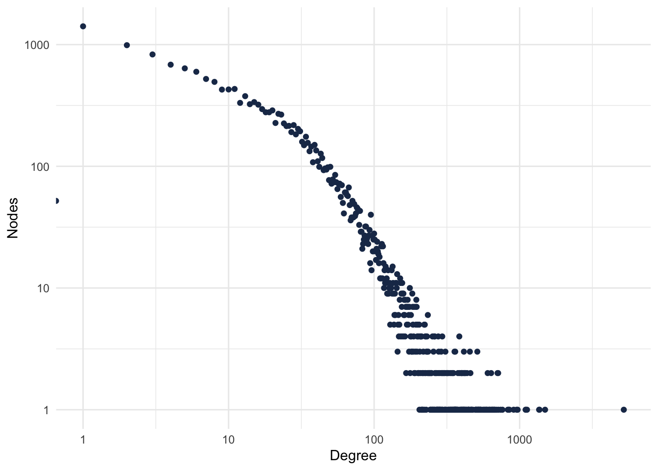

Figure 2.1: PPI Degree Distribution.

Most of the proteins have few connections, and very few proteins have lots of connections. Who’s that protein?

degree(gPPI) %>% 
  as.data.frame() %>% 
  arrange(desc(.)) %>%
  filter(. > 1000) 

##          .
## UBC   5199
## ETS1  1496
## GATA2 1369
## CTCF  1361
## EP300 1124
## MYC   1107
## AR    1099

2.1.4 Exercises

Now is your turn. Spend some minutes understanding the data and getting some familiarity with it.

1. What are the top 10 genes with the highest degree?

2. Are those genes connected?

2.2 Gene Disease Association

A Gene-Disease-Association (GDA) database are typically used to understand the association of genes to diseases, and model the underlying mechanisms of complex diseases. Those associations often come from GWAS studies and knock-out studies.

2.2.1 Commonly used data sources for GDAs

As PPIs, GDAs can be found from different sources and with different evidences for each Gene-Disease association. I list here some well-known databases for that.

• CTD – Curated scientific literature (Davis et al. 2020)

• OMIM – Curated scientific literature (McKusick 2007)

• DisGeNet – Based on OMIM, ClinVar, and other data bases (Piñero et al. 2019)

• Orphanet – Validated - and non-validated - GDAs

• ClinGen – Validated - and non-validated - GDAs (Rehm et al. 2015)

• ClinVar – Different levels of evidence (Landrum et al. 2019)

• GWAS catalogue – GWAS associations to diseases (Buniello et al. 2018)

• PheGenI – GWAS associations to diseases (Ramos et al. 2013)

• lncRNADisease – Experimentally validated lncRNAs in diseases (Chen et al. 2012)

• HMDD – Experimentally validated miRNAs in diseases (Huang et al. 2018)

2.2.2 Understanding a GDA dataset

We will use in this workshop Gene-Disease-Association from DisGeNet. It can be found here.

Similar to the PPI, let us first get some familiarity with the data, before performing any analysis.

Let’s read in the data and, again, do some basic statistics.

GDA = fread(file = 'data/curated_gene_disease_associations.tsv', sep = '\t')

head(GDA)

geneId	geneSymbol	DSI	DPI	diseaseId	diseaseName	diseaseType	diseaseClass	diseaseSemanticType	score	EI	YearInitial	YearFinal	NofPmids	NofSnps	source
1	A1BG	0.700	0.538	C0019209	Hepatomegaly	phenotype	C23;C06	Finding	0.30	1.000	2017	2017	1	0	CTD_human
1	A1BG	0.700	0.538	C0036341	Schizophrenia	disease	F03	Mental or Behavioral Dysfunction	0.30	1.000	2015	2015	1	0	CTD_human
2	A2M	0.529	0.769	C0002395	Alzheimer’s Disease	disease	C10;F03	Disease or Syndrome	0.50	0.769	1998	2018	3	0	CTD_human
2	A2M	0.529	0.769	C0007102	Malignant tumor of colon	disease	C06;C04	Neoplastic Process	0.31	1.000	2004	2019	1	0	CTD_human
2	A2M	0.529	0.769	C0009375	Colonic Neoplasms	group	C06;C04	Neoplastic Process	0.30	1.000	2004	2004	1	0	CTD_human
2	A2M	0.529	0.769	C0011265	Presenile dementia	disease	C10;F03	Mental or Behavioral Dysfunction	0.30	1.000	1998	2004	3	0	CTD_human

The first thing to notice is the inconsistency with the disease names, in order to be able to work with it, let’s first put every disease to lower-case.

Cleaned_GDA = GDA %>% filter(diseaseType == 'disease') %>%
  mutate(diseaseName = tolower(diseaseName)) %>%
  select(geneSymbol, diseaseName, diseaseSemanticType) %>%
  unique() 

dim(Cleaned_GDA)

## [1] 60478     3

dim(GDA)

## [1] 84038    16

numGenes = Cleaned_GDA %>% 
  group_by(diseaseName) %>%
  summarise(numGenes = n()) %>%
  ungroup() %>%
  group_by(numGenes) %>%
  summarise(numDiseases = n())

Let’s also understand the degree distribution of the diseases.

ggplot(numGenes) +
  aes(x = numGenes, y = numDiseases) +
  geom_point(colour = "#1d3557") +
  scale_x_continuous(trans = "log10") +
  scale_y_continuous(trans = "log10") +
  labs(x = "Genes", y = "Diseases")+
  theme_minimal()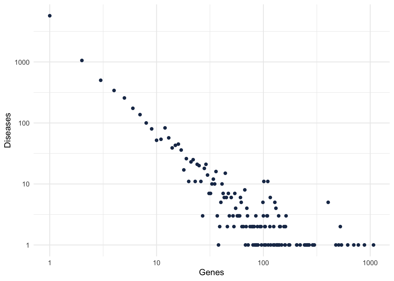

Figure 2.2: Gene-Disease degree distribution.

Because we want to focus in well studied diseases, and also that are known to be complex diseases, let’s filter for diseases with at least 10 genes.

Cleaned_GDA %<>% 
  group_by(diseaseName) %>%
  mutate(numGenes = n()) %>%
  filter(numGenes > 10)

Cleaned_GDA$diseaseName %>%
  unique() %>%  
  length()

## [1] 920

2.2.3 Exercises

Now is your turn. Spend some minutes understanding the data and getting some familiarity with it.

1. What are the top 10 genes mostly involved with diseases? What are those diseases?

2. What are the top 10 highly polygenic diseases?

3. What are the top 10 highly polygenic disease classes?

2.3 Drug-Targets

A druggable target is a protein, peptide, or nucleic acid that has an activity which can be modulated by a drug. A drug can be any small molecular weight chemical compound (SMOL) or a biologic (BIOL), such as an antibody or a recombinant protein that can treat a disease or a symptom.

2.3.1 Properties of an ideal drug target:

A drug-target has a couple of proprieties that are highly desired when constructing the drug (Gashaw et al. 2011):

• Target is disease-modifying and/or has a proven function in the pathophysiology of a disease.

• Modulation of the target is less important under physiological conditions or in other diseases.

• If the druggability is not obvious (e.g., as for kinases), a 3D-structure for the target protein or a close homolog should be available for a druggability assessment.

• Target has a favorable ‘assayability’ enabling high throughput screening.

• Target expression is not uniformly distributed throughout the body.

• A target/disease-specific biomarker exists to monitor therapeutic efficacy.

• Favorable prediction of potential side effects according to phenotype data (e.g., in k.o. mice or genetic mutation databases).

• Target has a favorable IP situation (no competitors on target, freedom to operate).

2.3.2 Commonly used data sources for GDAs

There are a couple of really good data sets that report drug-target interactions, I list here three good examples:

1. DrugBank (Wishart et al. 2006; Wishart et al. 2017)

2. CTD (Davis et al. 2020)

3. Broad Institute Drug Repositioning Hub (Corsello et al. 2017)

2.3.3 Understanding a Drug-Target dataset

For this workshop, we will use the drug bank drug-target dataset, and it can be found here. This dataset is from Drug-Bank, and has been previously parsed for your convenience. The original file is an XML file, and needs to be carefully handled to get information needed.

Similar to the PPI and the GDA, let us understand a little bit of the data set, and what kind of information we have here.

DT = fread(file = 'data/DB_DrugTargets_1201.csv')

head(DT)

i	ID	Name	Started_commer	Ended_commer	ATC	State	Approved	Gene_Target	DB_id	name	organism	Type	known_action
1	DB00001	Lepirudin	1997-03-13	2012-07-27	B01AE	liquid	approved	F2	BE0000048	Prothrombin	Humans	Polypeptide	yes
2	DB00002	Cetuximab	2004-06-29	NA	L01XC	liquid	approved	EGFR	BE0002098	Low affinity immunoglobulin gamma Fc region receptor II-a	Humans	Polypeptide	unknown
2	DB00002	Cetuximab	2004-06-29	NA	L01XC	liquid	approved	FCGR3B	BE0002098	Low affinity immunoglobulin gamma Fc region receptor II-a	Humans	Polypeptide	unknown
2	DB00002	Cetuximab	2004-06-29	NA	L01XC	liquid	approved	C1QA	BE0002098	Low affinity immunoglobulin gamma Fc region receptor II-a	Humans	Polypeptide	unknown
2	DB00002	Cetuximab	2004-06-29	NA	L01XC	liquid	approved	C1QB	BE0002098	Low affinity immunoglobulin gamma Fc region receptor II-a	Humans	Polypeptide	unknown
2	DB00002	Cetuximab	2004-06-29	NA	L01XC	liquid	approved	C1QC	BE0002098	Low affinity immunoglobulin gamma Fc region receptor II-a	Humans	Polypeptide	unknown

Cleaned_DT = DT %>% 
  filter(organism == 'Humans') %>%
  select(Gene_Target, Name,ID, Type, known_action) %>%
  unique() 

dim(Cleaned_DT)

## [1] 22931     5

dim(DT)

## [1] 26817    16

head(Cleaned_DT)

##    Gene_Target      Name      ID        Type known_action
## 1:          F2 Lepirudin DB00001 Polypeptide          yes
## 2:        EGFR Cetuximab DB00002 Polypeptide      unknown
## 3:      FCGR3B Cetuximab DB00002 Polypeptide      unknown
## 4:        C1QA Cetuximab DB00002 Polypeptide      unknown
## 5:        C1QB Cetuximab DB00002 Polypeptide      unknown
## 6:        C1QC Cetuximab DB00002 Polypeptide      unknown

TargetDist = Cleaned_DT %>% 
  group_by(Gene_Target) %>%
  summarise(numDrugs = n()) 

DrugDist = Cleaned_DT %>% 
  group_by(ID) %>%
  summarise(numTargets = n()) 

ggplot(TargetDist) +
  aes(x = numDrugs) +
  geom_histogram(colour = "#1d3557", fill = "#a8dadc" ) +
  labs(x = "Targets", y = "Drugs")+
  theme_minimal()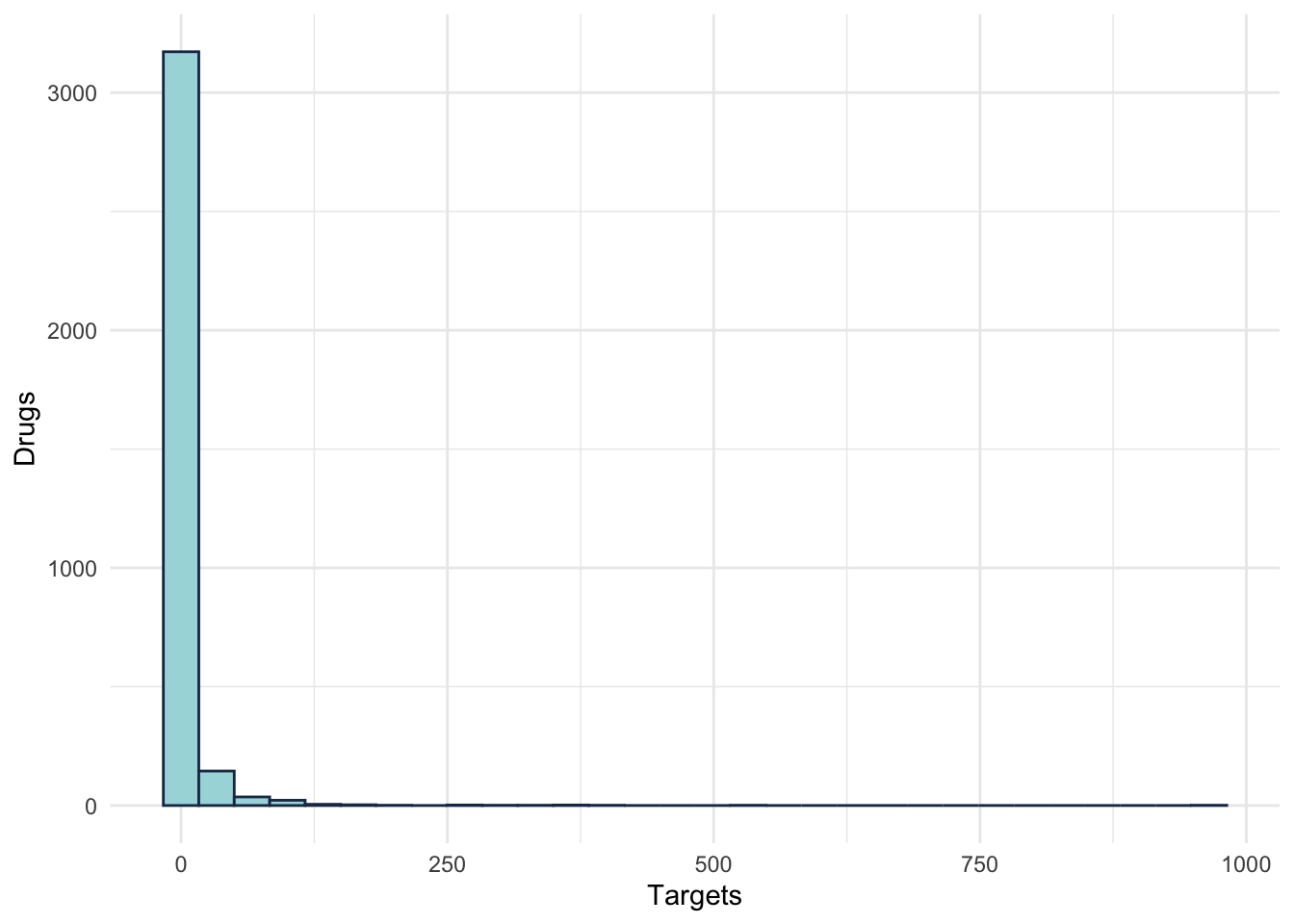

Figure 2.3: Target distribution

Which Target is the most targetted gene?

TargetDist %>%
  arrange(desc(numDrugs)) %>%
  filter(numDrugs > 400)

## # A tibble: 2 x 2
##   Gene_Target numDrugs
##   <chr>          <int>
## 1 CYP3A4           966
## 2 ABCB1            524

ggplot(DrugDist) +
  aes(x = numTargets) +
  geom_histogram(colour = "#1d3557", fill = "#a8dadc" ) +
  labs(y = "Targets", x = "Drugs")+
  theme_minimal()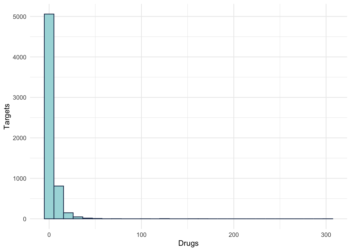

Figure 2.4: Drug distribution

2.3.4 Exercises

Let us understand a little bit more about the data.

1. What are the top 10 genes mostly targeted by drugs? Are they types are they mostly?

2. What are the top 10 most promiscuous drugs? What are their indication?